Automated Turret

January 2025 - April 2025

GitHub Repository

Introduction

My sixth major course at USNA was EW309 (System Modeling and Simulation). We pursued a project starting from the problem statement to the final prototype and report.

The final project was to design and build a turret that could automatically track and fire at a target.

Demo Video

Final Report

Abstract — The EW309 automated turret design project aimed to develop a fully autonomous control system for the Sentry Turret, integrating motor control, computer vision, and ballistics analysis to accurately detect, aim, and engage static circular targets with a minimum accuracy of 95%. The project was based on applications in defense, law enforcement, and industrial automation, and it highlighted the critical engineering challenges associated with autonomous targeting, precise motor control, and feedback systems. The final turret design employed a dual-axis actuation system powered by DC motors and controlled via a custom-built circuit using a Raspberry Pi Pico microcontroller. Target detection used the Luxonis OAK-1 Lite camera paired with a YOLOv11 based neural network, and achieved classification and localization of colored targets within a given board space and with varying conditions. Performance evaluations demonstrated that the turret can successfully target specified circles and discriminate between valid targets and decoys with steady-state errors within ±0.5°. Ballistics testing across distances between 10 feet and 20 feet quantified system biases and precision, confirming the turret’s capability to reliably meet specified performance criteria. These results reinforce the effectiveness of classical control methods combined with advanced computer vision in an autonomous turret system.

Introduction

Automated turrets have evolved in recent years, including integrating computer vision and custom motor control to improve targeting accuracy and responsiveness. This project focuses on designing an electrical control system for a prefabricated Sentry Turret that incorporates the concepts of the United States Naval Academy’s Robotics and Control Engineering major. By using a combination of computer vision, motor control, and feedback loops, the turret will autonomously identify and engage targets within its field of view with at least 95% overall accuracy. This section details the motivation behind the project, the problem statement, and the background research that informs the design and implementation of the turret system.

Motivation

Autonomous turrets have significant applications across various industries, including military, law enforcement, and consumer products. In the military, autonomous targeting systems enhance security by providing rapid threat assessment and response with minimal human input or casualties. The ability to identify and neutralize targets while avoiding unintended harm to noncombatants is crucial both ethically and operationally. Beyond defense and law enforcement, autonomous turrets are increasingly used in commercial and research settings, such as industrial automation, wildlife monitoring and management, and robotics competitions. The growing sophistication of computer vision and automated control systems has enabled more precise and accurate targeting, reducing reliance on human operators and increasing overall efficiency. This project addresses key challenges in target identification, motor control, and feedback loops, reinforcing fundamental concepts in robotics, control theory, and computer vision. By engaging with these technical challenges, students gain a deeper understanding of how autonomous systems operate, fostering both technical proficiency and critical thinking.

Problem Statement

Design, implement, and test an autonomous method of controlling a prefabricated Sentry Turret. The method should enable the turret to autonomously detect and hit two circular static targets of a specified size and color with 95% accuracy. The turret should be able to distinguish between its target and decoys of many sizes and colors, including the same size or color as the target. The gun itself will operate in a stationary position with an unobstructed view. The turret should be able to detect two targets within the full field of view of the gun mounted camera, aim itself, and fire accurately at those targets within 15 seconds. The system must also provide diagnostics at the end of each trial including the final steady-state error for pitch and yaw rotations and how many shots the turret intended to take.

Background Research

Modern automated turret designs rely on a camera for target detection and motor actuators to orient the gun. For example, [1] demonstrated a system using a webcam and two stepper motors to aim a toy gun, as illustrated in Fig. 1. The turret implements a motion detection algorithm to detect any movement within the camera’s field of view. If motion is detected, the system will calculate the necessary rotation angle and required motor steps to aim at its general location. This approach offers a cheap and easily replicable design, but the target acquisition software remains rudimentary.

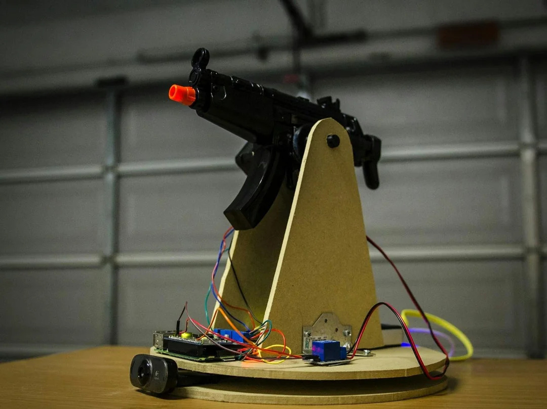
Figure 1: Motion detecting Nerf gun turret [1]

Advancements in computer vision explore facial recognition and the use of color filters [2] for targeting, as illustrated in Fig. 2. The method proposed can detect and target multiple colors or faces with the use of Hue, Saturation, and Value color filtering. Alternative methods incorporate human detection capabilities using histogram of oriented gradient (HOG) and support vector machine (SVM) classifiers [3]. Even with the advances in computer vision algorithms, these systems fail to implement a target discriminating capability, shooting anything that moves.

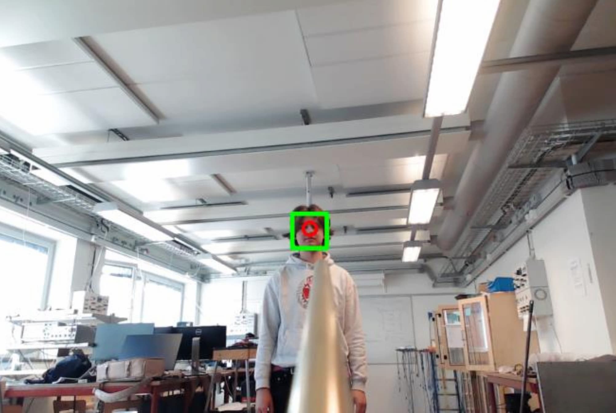
Figure 2: Face detecting laser pointer turret [2]

To overcome the limitations of non-discriminatory target acquisition, recent work focuses on targeting the largest object within the camera's field of view [4]. Should a blue object get within the camera’s field of view, the turret will reach the desired servo angles to aim a laser at it. If there are multiple blue objects detected, the turret will aim at the largest target. The main advantage of the design is its ability to discriminate between different targets based on their size. However, the target acquisition program is still quite limited as it only locates blue objects. Providing the user with greater control over target selection would enhance the automated turret's ability to distinguish and prioritize firing at specified targets.

Several turret actuation methods rely on servo motors [2],[3],[4], as illustrated in Fig. 3. Servo motors implement a built-in position controller for motor actuation. While this might work with small turret designs, servo motors tend to not exist at large sizes. To scale this approach for actuating larger guns, a custom motor position control loop would be necessary [5]. An additional sensor (like an encoder) would be required to measure the motor’s position and an additional controller must be developed to calculate the input voltage.

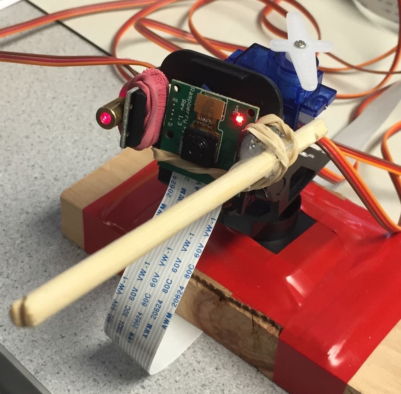
Figure 3: Servo motor actuated turret [4]

To address the limitations of previous works [1],[2],[3],[4] this report will encompass an automated turret system enabling the user to specify the characteristics of the targets to fire at and utilize an easily scalable motor controller. By utilizing advancements in computer vision, the turret can distinguish between pre-specified targets and decoys. Additionally, by utilizing a classical approach towards motor position control, this method can be easily reproduced at scale.

Turret Actuation

The turret’s actuation system is made up of three main subsystems: a laptop for user/programmable control, a turret board which handles interpreting signal commands and power, and the turret body. These processes are depicted in Fig. 4 and all code can be found in the GitHub repo.

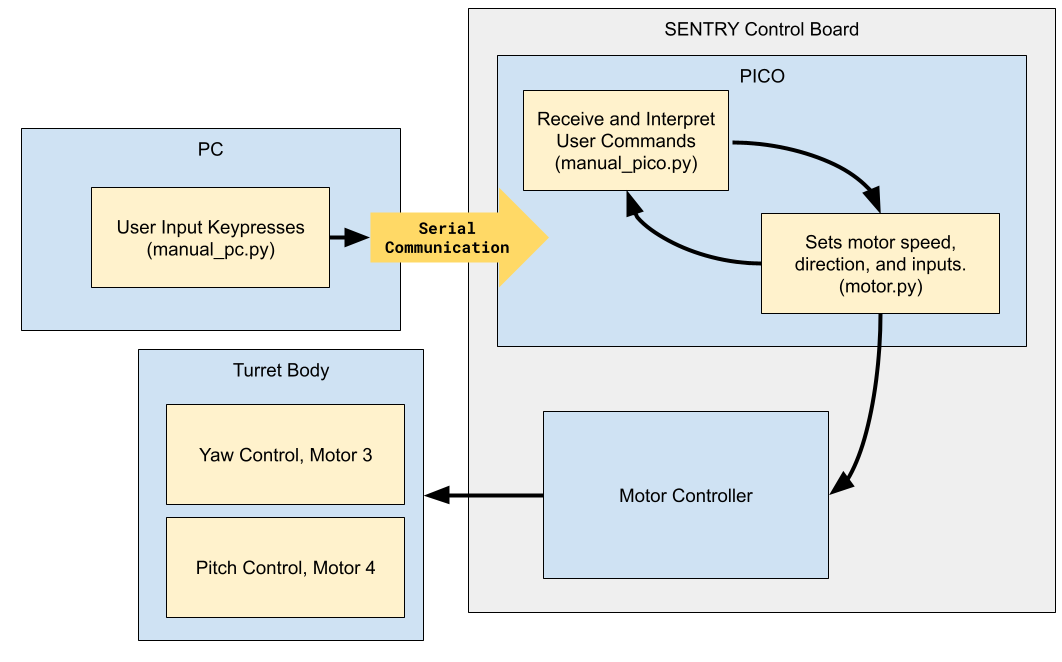
Figure 4: Operational block diagram for actuation phase

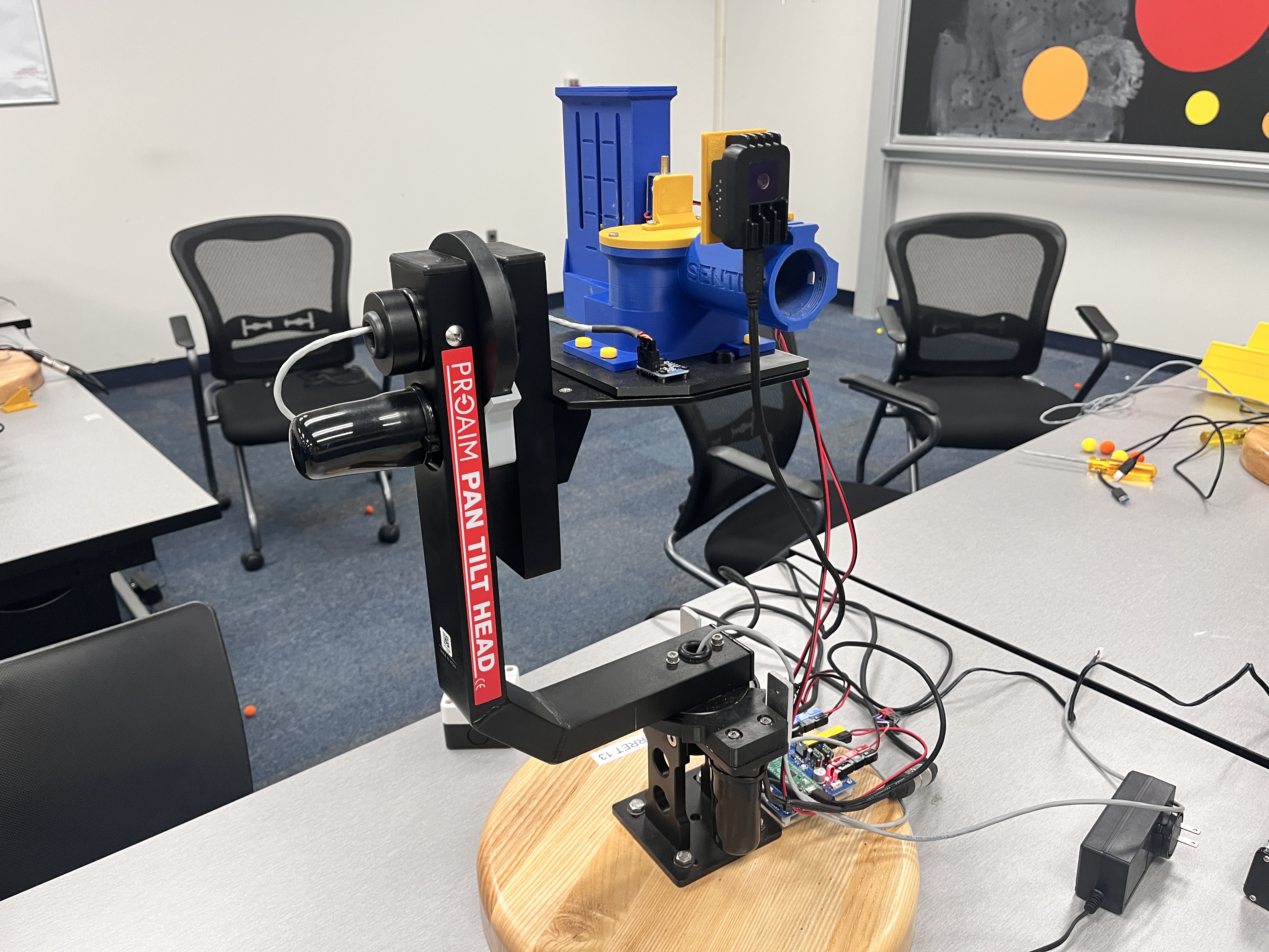
The turret body is a repurposed Proaim Sr. Pan Tilt Head [6] operating on two axes, yaw and pitch. A custom motor control board replaces the default control box, enabling direct interfacing with the motors. The tilt head is modified to operate in a 180° range with a physical stop and the pan head can operate without limitations, captured in Fig. 5. It has two brushed, high torque DC motors that can operate between 6°/sec at 4VDC and 51°/sec at 12VDC, according to Proaim [6]. Both motors are using far less than their maximum load of 16.5lbs. The custom circuit board, shown in Fig. 6, connects two systems: a Raspberry Pi PICO microcontroller, which manages control logic and interprets commands from the laptop, and two motor drivers that power the motors and control their speed and direction. The two ROHM BD62120AEFJ motor drivers can operate between 8VDC and 24VDC [7], are powered via a 12VDC power supply and are used to control both the yaw and pitch motors.

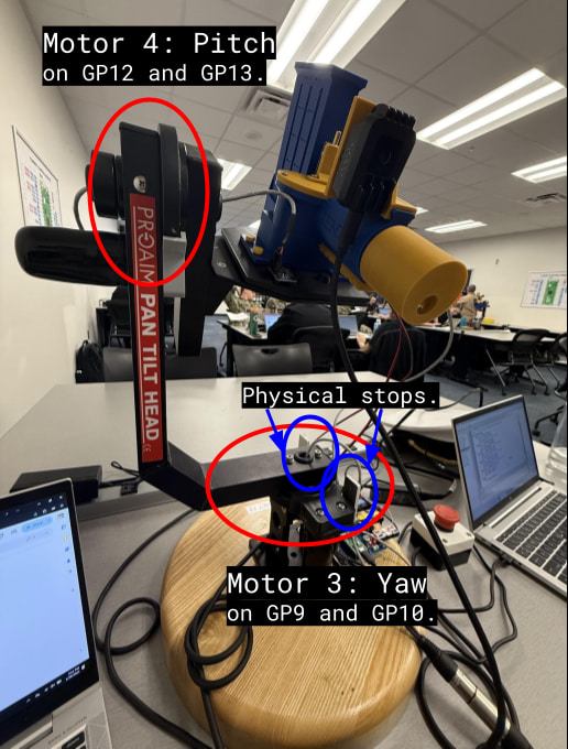
Figure 5: Turret motor locations

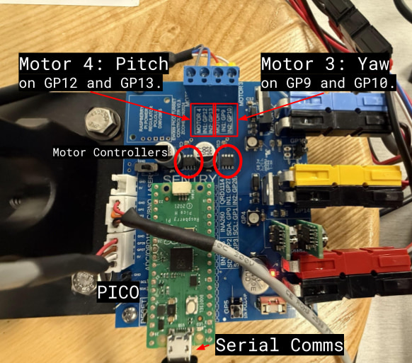
Figure 6: Board layout and motor wiring

The main advantage for using this motor driver is its ability to control high power (12VDC) motors with low power (3.3VDC) pulse width modulation (PWM) logic from the PICO microcontroller [8]. The motor driver is a standard H-bridge that allows control over polarity of the load, which in turn, allows control over the direction of the motors. Motor direction and speed is facilitated via two low power PWM input pins, IN1 and IN2. Turning IN1 on and IN2 off causes clockwise rotation and turning IN1 off and IN2 on causes counterclockwise rotation. Speed is directed via the PWM duty cycle through each pin. A 100% duty cycle would result in full power (12VDC) and a 0% duty cycle would result in no power (0VDC). The PWM frequency of 1kHz was selected to balance audible motor noise and efficient operation. This motor driving process is managed by the motor class, motor.py, in the GitHub repo.

In order to control the turret, the PC communicates movement commands to the PICO over a serial port. The PICO then decides which motor to actuate and the polarity of voltage to achieve the desired motor rotation. Finally, the microcontroller sends PWM signals to the motor controllers to power the motors for yaw and pitch actuation.

The user can use the left arrow key, right arrow key, up arrow key, and down arrow key to control the orientation of the turret and use the space key to stop the motors. Upon key press, the laptop will send the respective movement command over serial to the PICO (manual_pc.py). When the microcontroller receives the commands "RIGHT" or "LEFT," it interprets them as clockwise or counterclockwise rotation, respectively. Via pins GP9 (IN1) and GP10 (IN2), the microcontroller will instruct the motor controller to apply 12V DC at a 60% duty cycle to the yaw motor. The same is true for commands “UP” or “DOWN,” but for the pitch motor at GP12 (IN1) and GP13 (IN2). A 60% duty cycle was chosen for a controlled yet responsive motor speed. The “SPACE” command locks both motors by setting the IN1 and IN2 duty cycle to 100% (manual_pico.py).

The greatest difficulty experienced was getting the laptop to detect keyboard presses and send them to the PICO via serial. The initial attempt used MATLAB for keyboard control to allow for easy integration of data collection and analysis. Unfortunately, MATLAB does not offer a straightforward solution for this, so an alternative approach was implemented using the Python keyboard library [9]. This allowed key presses to be detected using the is_pressed() method within a while loop. While granting easier control of the turret, it may require the use of Python data analysis tools instead of MATLAB. Looking forward, it's important to be flexible during problem-solving and avoid relying too heavily on familiar approaches.

Position Sensor

The turret has a BNO055 9-axis inertial measurement unit (IMU) [10] which consists of triaxial accelerometer to measure linear acceleration, a triaxial gyroscope to measure angular velocity, and a triaxial magnetometer to measure the sensor's orientation relative to magnetic north. Since the turret needs a motor position controller to aim at the target, orientation and angular velocity measurements are required. Orientation measurements are used for the calculation of the error between current and desired motor positions, and angular velocity data will be utilized for system identification (plant transfer function estimation).

Although only orientation and angular velocity are required, relying solely on the gyroscope is insufficient. Gyroscope measurements are inherently noisy, sensitive to temperature variations, and do not directly provide orientation. Instead, orientation is derived by integrating angular velocity, which accumulates sensor bias over time, leading to drift. To counteract this, sensor fusion combines data from the accelerometer, gyroscope, and magnetometer, yielding a more accurate state estimation. The accelerometer and magnetometer improve orientation measurements by referencing constant external vectors: the gravity vector from the accelerometer and magnetic north from the magnetometer.

The BNO055 IMU communicates to the PICO via Inter-Integrated Circuit (I2C) on pins GP2 and GP3. This is pictured in Fig. 7 with the additional two wires being the sensor’s ground and 5V power.

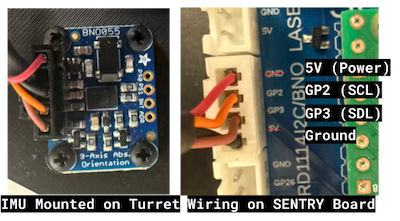
Figure 7: BNO-055 IMU Wiring Diagram and Mounting

GP2 (orange wire) is a serial clock line (SCL), crucial for synchronizing communication between the PICO and IMU. It does this by sending pulses at regular intervals, with each pulse indicating when each bit of data is transmitted via GP3 (brown wire) or the serial data line (SDA). Using the Adafruit BNO055 library [11], the PICO receives the yaw, roll, and pitch position in degrees and velocity in degrees per second using the euler() and gyro() methods respectively. The yaw and pitch data (roll data discarded) are then streamed over serial to the PC using a formatted print statement. The PC receives that information in a data array which it decodes into yaw and pitch position data and velocity data, for a total of four lists storing data as it is recorded.

The streamed data is published at a constant rate of 10 Hz by using a while loop and time.sleep(0.1). Collecting measurements at 10 Hz should be fast enough for most motor control designs and reading at equal time intervals is crucial for accurate control calculations. A PID controller, for example, requires integrals and derivatives. Inconsistent measurement intervals distort these calculations, potentially accumulating errors and hindering the controller's ability to reach the desired position.

To enable concurrent reading and writing to the serial port, the PICO leverages its dual-core Arm Cortex-M0+ processor [8], executing each process to a separate thread. This is done via the _thread MicroPython library [12] and allows the turret to simultaneously receive keyboard movement commands from the laptop while publishing constant IMU data back to it. Fig. 8 illustrates the process from start to finish, noting that the data collection process continuously loops until “q” is pressed. The code for this process can be found in manual_IMU_pico.py in the GitHub repo.

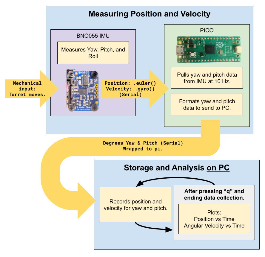
Figure 8: Component Operations Diagram for serial communication

Fig. 9 displays a plot of the turret’s position and velocity over a testing period of five seconds using the Matplotlib library [13] in manual_IMU_pc.py script. The test shifted the turret clockwise then counterclockwise (yaw), stopped, then tilted the turret down then back up (pitch), which agrees with the Position vs. Time plot. Each time the turret changes direction in either direction, the velocity shifts quickly to a constant speed of about ±40 deg/s as seen in the Angular Velocity vs. Time plot. This consistency in moving in either the clockwise or counterclockwise direction will make it easier for system identification. Instead of having to calculate four different transfer functions for movement in all four directions, only two or maybe even one transfer function would be required to model the DC motor turret system.

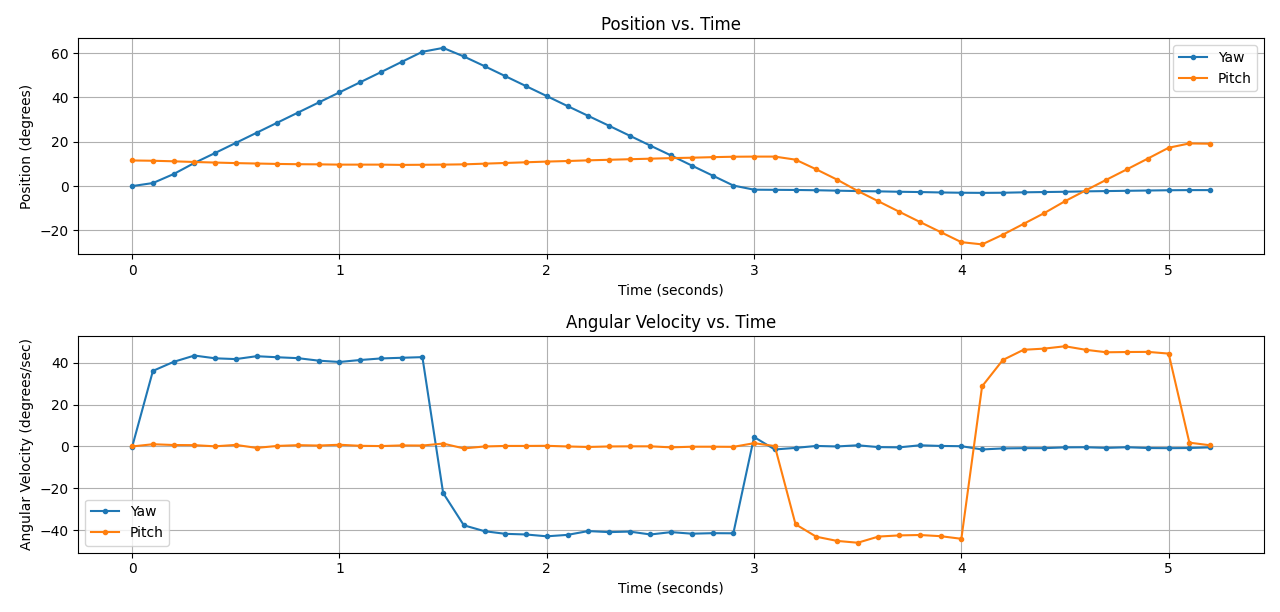
Figure 9: Plot of Position vs. Time and Angular Velocity vs Time for turret motor actuation

Initially, getting two-way serial communication between the PICO and laptop proved to be difficult. The original approach utilized the Python asyncio library for concurrent processing, but the _thread library was more straightforward to implement and provided better documentation. This allowed the PICO to manage two independent processes, serial reading and writing, to operate simultaneously on different threads.

Additional issues occurred while rotating across the turret’s centerline, when the PC recorded a dramatic jump from 0° to 360°. This large shift would make it difficult to implement a position controller which requires a smooth transition between angles. A sudden jump, representing the same relative position, can confuse the controller and lead to erratic behavior. To mitigate this issue, a “wrap to pi” function was implemented to map the data to a continuous range from -180° to 180°. This function can be seen in manual_IMU_pico.py in the GitHub repo.

During testing, a frequent problem arose when the PICO script would time out if a keyboard command was not received. If the user did not send commands quick enough, there was a high chance the script would break. Initially, a simple sleep command allowed enough time to press a key after code execution, but a more robust solution was implemented utilizing a while loop. The program now loops continuously until a serial command triggers its exit, allowing the remaining code to execute.

Controller Design

This section of the report outlines the process of data collection, transfer function derivation, system response analysis, and controller development for the yaw and pitch motors. The System Modeling section covers data collection and transfer function derivation, while the Deadzone Compensation section explains how stiction in the DC motors was addressed. The Yaw and Pitch Controller Design section details the approach used to develop a position controller. To enhance system performance, a Proportional-Integral (PI) controller was implemented. The PI controller adjusts the control input based on the current error (proportional) and the accumulation of past errors (integral), ensuring immediate error correction while eliminating steady-state error. Finally, the Performance Evaluation section assesses the controller's effectiveness, comparing its performance to design expectations and outlining any modifications made to improve the system.

System Modeling

The objective of system modeling is to develop a mathematical model of the Sentry Turret motors, which is crucial for evaluating its dynamics before designing a controller. The system model provides transfer functions to analyze and predict the turret’s behavior based on a given input. For this setup, the velocity transfer function was derived using a first-order system approximation of the DC motor turret system. While more accurate models exist for representing the system, a first-order approximation is sufficient for determining the appropriate controller type and calculating initial control gains based on a design point.

Data collection was carried out using controlled, repeatable, and time-based trials to model the turret’s dynamics. First-order system analysis was performed by examining the step response for each motor. A step response with a 30% duty cycle was selected to provide enough voltage to initiate motor movement, while keeping the speed low enough to allow for accurate data measurements from the 10Hz IMU. Each motor received a one-second step input, using the time.sleep() method, to ensure it reached its final value. During the whole trial, the PICO recorded angular velocity and angular position from the IMU using the gyro() and euler() methods, respectively. Measurements were taken at equal time intervals to reduce the risk of missing critical changes in the system’s behavior and simplify the transfer function estimation. Each motor was powered individually in both directions, clockwise (CW) and counterclockwise (CCW) for yaw, and up and down for pitch, as shown in Fig. 10 and performed via the calc_TF_pico.py and calc_TF_pc.py scripts in the GitHub repo.

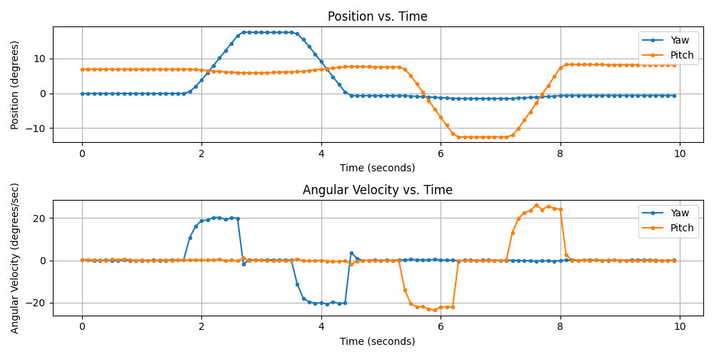
Figure 10: Position and angular velocity step response for yaw and pitch motors at 30% duty cycle

Using this data, first-order system analysis can be performed to estimate the motor’s transfer function. The velocity transfer function represents how the turret's angular velocity in deg/s responds to a given motor input in volts and is given by,

$G_{vel}(s)=\frac{b}{s+a}.$

(1)

The position transfer function represents how the turret’s position in degrees responds to a given motor input in volts and can be derived by taking the integral of the velocity transfer function,

$G_{pos}(s)=\frac{b}{s(s+a)}.$

(2)

The coefficients $a$ and $b$ are found via the calc_TF_data_anlaysis.py script by analyzing the velocity step response data, as illustrated in Fig. 11. The blue line represents the step response and black line denotes the start of the given motor step input. The final value, $F_v$, (red line) was calculated by taking the average of the last four values of the step response to compensate for any noise within the velocity measurement. The 63% final value is denoted by the magenta line and was used for determining the system's time constant, $\tau$, (green line) or the time it takes for the motor to reach 63% of its final velocity.

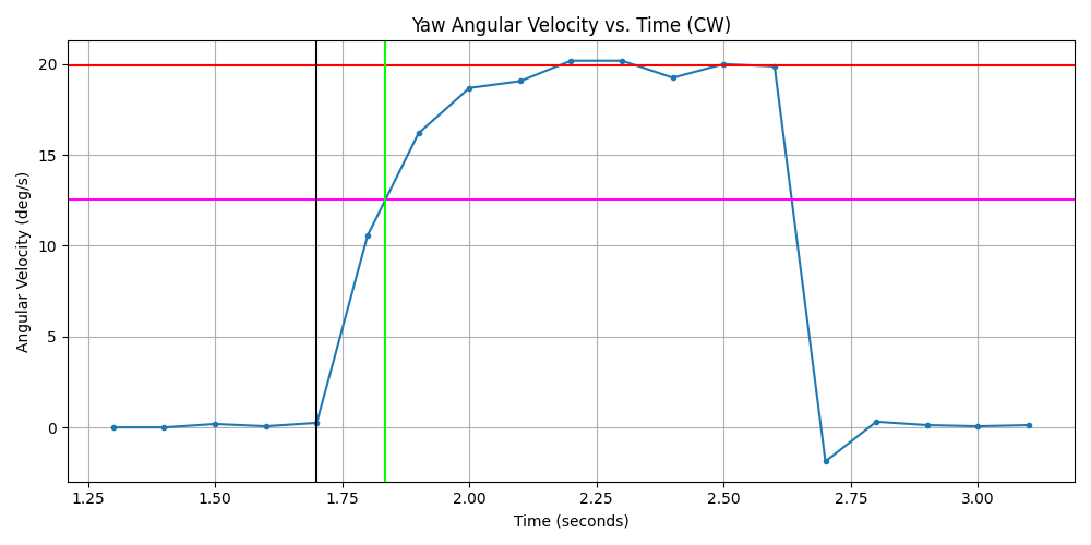
Figure 11: Step Response of Yaw Angular Velocity showing transient response, final velocity, time constant, and t=0

The coefficient $a$ for the first order system can be calculated by,

$a=\frac{1}{\tau},$

(3)

where $\tau$ represents the time constant in seconds. The coefficient $b$ can be calculated by

$b=\text{SSG}*a,$

(4)

where the SSG (Steady State Gain) is calculated by

$\text{SSG}=\frac{F_v}{\text{Step Magnitude}}.$

(5)

The step magnitude was 3.6 volts which was achieved via a 30% duty cycle of 12 volts.

These steps were repeated for each of the four movements: CW, CCW, up, and down. For each motor, one velocity and one position transfer function were calculated by averaging the $a$ and $b$ coefficients between its complementary movements, CW and CCW for yaw, and up and down for pitch. This averaging process reduces the number of estimated transfer functions per motor, assuming that the yaw and pitch motors exhibit similar behavior in both directions.

The transfer functions derived for yaw velocity, yaw position, pitch velocity, and pitch position are given by the following equations. Of note, the position transfer functions are second order as position is not measured directly from the IMU but rather calculated by taking the integral of velocity transfer function. The yaw velocity transfer function is,

$G_{vel,yaw}(s)=\frac{44.52}{s+7.979},$

(6)

and the corresponding yaw position transfer function is,

$G_{pos,yaw}(s)=\frac{44.52}{s(s+7.979)}.$

(7)

Similarly, the pitch velocity transfer function is,

$G_{vel,pitch}(s)=\frac{55.28}{s+8.189},$

(8)

and the pitch position transfer function is,

$G_{pos,pitch}(s)=\frac{55.28}{s(s+8.189)}.$

(9)

The step response for the estimated velocity transfer function compared to the recorded angular velocity of both yaw (6)and pitch (8) are illustrated in Fig. 12. The yaw angular velocity transfer function in both the CW and CCW directions track the step responses closely. The same can be said for the pitch angular velocity transfer function. Upon closer inspection, the yaw angular velocity step response for the CW direction reaches a final value of 19.9 deg/s whereas the step response in the CCW direction exceeds -20 deg/s at -20.17 deg/s. This difference in motor dynamics is likely associated with slight imperfections in the manufacturing process and uneven wear.

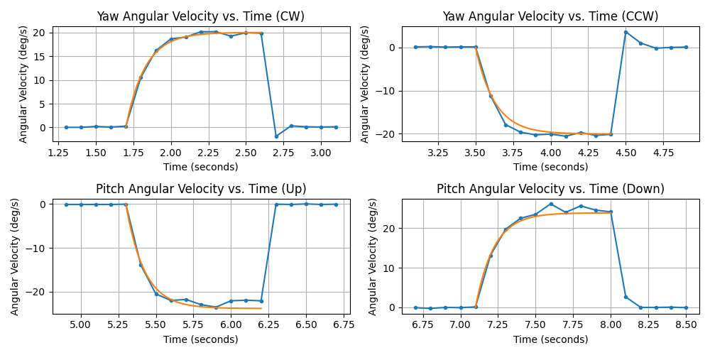
Figure 12: Angular Velocity vs Time plots for transfer function evaluation at 30% duty cycle

Furthermore, the pitch angular velocity step response in the up direction reaches a final value of -22.6 deg/s, with the down direction reaching 25.0 deg/s. The increase in angular velocity between the yaw and pitch motors is associated with the lighter load. The yaw motor has to move the full pan/tilt mechanism whereas the pitch motor only has to move the gun. The discrepancies of angular velocity between the up and down direction are the result of slight imbalances of the gun placement. While the gun is balanced within reason, its center of gravity is not perfectly even with the center of the pan/tilt mechanism. As a result, the pitch angular velocity transfer function appears to exceed the final value for the up direction and slightly undershoot the final value for the down direction.

The step response of the estimated position transfer function compared to the observed position for both yaw (7) and pitch (9) are illustrated in Fig. 13. Examination of the yaw position transfer function step response reveals a close fit with the logged position data. In the CW direction, the estimated response closely follows the recorded position. By contrast, the CCW direction estimated response slightly undershoots the recorded position. The difference in performance can be explained by the associated velocity transfer function behavior. In the clockwise direction, it closely tracks the final velocity, whereas in the counterclockwise direction, it underestimates it. This leads to inaccuracies in the estimated position, as a lower (or higher) estimated velocity naturally results in a lower (or higher) estimated position. The pitch motor's estimated position response also exhibits this relationship with the velocity transfer function. In this case, upward movement shows near-perfect tracking with the recorded position, while downward movement reveals a moderate undershoot. The same comparison can be made with the associated velocity transfer function response as illustrated in Fig. 12.

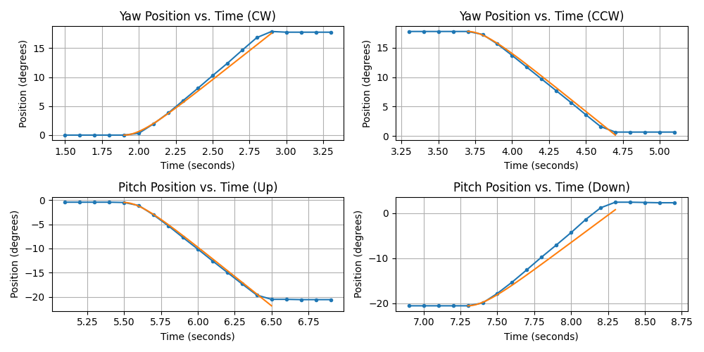
Figure 13: Position vs Time plots for transfer function evaluation at 30% duty cycle

To evaluate the robustness of the estimated transfer function, a step response at a 100% duty cycle was conducted to assess how closely the predicted position response matched the observed response at a different speed, as shown in Fig. 14.

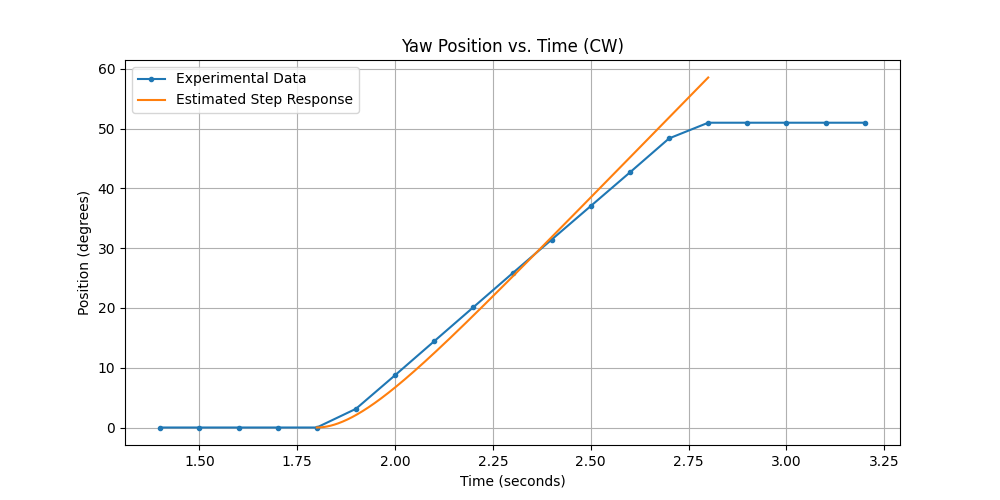
Figure 14: Position vs Time plots for transfer function evaluation at 100% duty cycle

While the estimated angular velocity and position transfer function for both the yaw and pitch motors were not perfect, they serve as an adequate approximation of the system. A well-designed motor controller can effectively handle these variations and achieve stable performance. Future work could focus on refining the model with 2nd order system identification or even null space adaptive identification techniques [14].

While deriving the transfer function, several challenges arose. One minor difficulty was determining the time constant accurately. To estimate it, interpolation between measured values was needed to approximate 63% of the steady-state value. Increasing the streaming rate would have improved accuracy, but this introduced another problem discussed in the next paragraph. Although interpolating data in MATLAB was straightforward, doing so in Python required more effort and troubleshooting. Ultimately, the NumPy documentation [15] provided clear guidance on how to interpolate between two data points.

The most challenging issue stemmed from an unexpected error caused by the gyroscope streaming at a rate exceeding 100 Hz. The BNO055 has a limited output rate, and requesting a sampling rate that was too high caused the gyroscope to report incorrect angular velocity. As a result, the transfer function aligned with the velocity step response, since it was based on that data, but failed to accurately reflect the position step response. During troubleshooting, it was determined that reducing the sampling rate to 10 Hz resolved the issue, necessitating interpolation of the velocity data.

It is also important to evaluate the resulting time constants for both the yaw and pitch angular velocity step responses. As a rule of thumb, the controller's sampling rate should between 5-10 times faster than the system's time constant to achieve stable control. With both the yaw and pitch responses yielding a time constant of 0.12 seconds, the ideal update rate would between 42-83 Hz. A sampling rate of 60 Hz was selected for the controller, as it strikes a balance within the specified range while adhering to the limitations of the BNO055 data rate.

Deadzone Compensation

Due to stiction in the DC motors, a minimum duty cycle or voltage is required for movement. If the controller's input falls within this deadzone, the turret may fail to respond, leading to steady-state error. Therefore, it is crucial to determine the deadzone duty cycle, or the minimum duty cycle needed to initiate motor movement.

To identify this threshold, the find_deadzone_pc.py and find_deadzone_pico.py scripts incrementally increase the duty cycle and corresponding motor voltage until motion is observed. The user specifies the rotation direction by pressing an arrow key (e.g., the up arrow to move the turret up) and repeatedly presses the key to raise the duty cycle. A starting duty cycle of 15% was chosen, as it falls below the observed deadzones for both the yaw and pitch motors. Once movement is detected, the user presses the space key to stop the turret before repeating the process for another motor or direction. This process is illustrated in Fig. 15, where yaw CW, yaw CCW, pitch down, and pitch up were tested in that sequence.

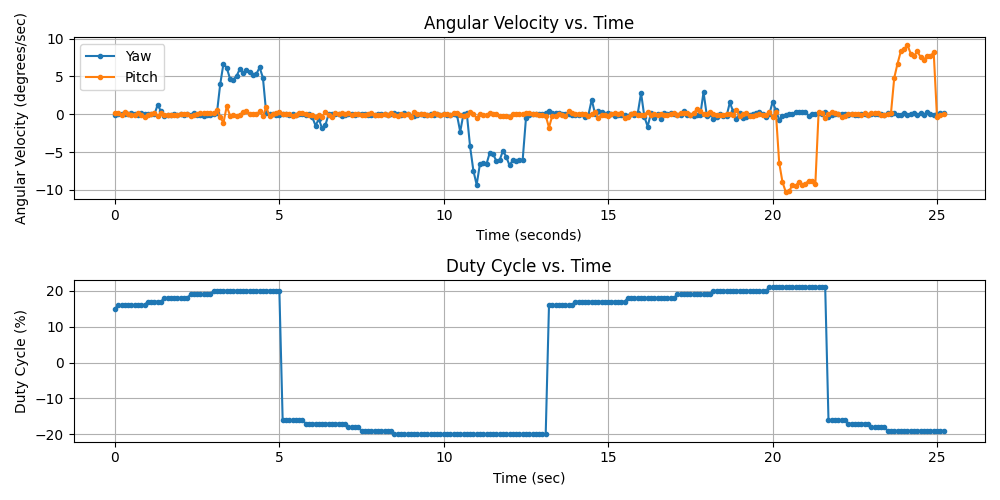
Figure 15: Motor Voltage and Angular Velocity vs Time plots finding deadzone duty cycle

The find_deadzone_data_analysis.py script analyzed the collected data to extract the last recorded duty cycle for each movement, identifying the deadzone duty cycles as 20%, 20%, 21%, and –19% for yaw CW, yaw CCW, pitch down, and pitch up, respectively. Using these estimated deadzone values, the controller compensates for the deadzone by adding the positive deadzone duty cycle to any input above zero (positive duty cycle) and subtracting the negative deadzone duty cycle from any input below zero (negative duty cycle). Although this method introduces nonlinearity into the system, the controller remains robust due to negative feedback, even though it is designed for a linear system. The code implementation can be found in the GitHub repo.

Yaw and Pitch Controller Design

The turret must accurately aim at two targets and hit them within a 15-second time frame. To align with the grading rubric, the chosen design specifications include a settling time of 1.25 seconds, an overshoot of less than 20%, and a steady-state error within ±0.61° (explanation of the angle steady-state error is detailed in the GitHub repo). However, the overshoot requirement is not strict, as the primary focus is on achieving fast target acquisition and minimal steady-state error.

Given the presence of a constant disturbance due to motor friction, a Proportional-Integral (PI) controller was selected to ensure zero steady-state error. The PI controller is modeled as,

$u(t)=K_pe(t)+K_i\int_{0}^{t}e(\tau)d\tau,$

(10)

where $u(t)$ represents the output duty cycle and $e(t)$ represents the error,

$error=desired\;position-current\;position,$

(11)

$K_p$ and $K_i$ are the proportional and integral gains respectively. $K_p$ provides proportional correction based on the error and $K_i$ eliminates steady state error.

By taking the Laplace of $u(t)$, the following input function can be derived in the frequency domain,

$U(s)=K_p\left[E(s)+\frac{K_i}{K_p}\frac{E(s)}{s}\right].$

(12)

After rearranging terms, the transfer function from $E(s)$ to $U(s)$ is as follows,

$\frac{U(s)}{E(s)}=K\frac{s+z_{PI}}{s},$

(13)

where $K$ is equivalent to $K_p$ and $z_{PI}$ is equivalent to $\frac{K_i}{K_p}$. Using the position transfer function for both yaw (6) and pitch (8), the negative feedback loop illustrated in Fig. 16 can be implemented.

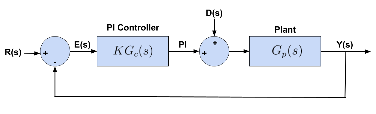
Figure 16: PI control block diagram

The signal, $R(s)$, refers to the reference or desired position state and $Y(s)$ represents the actual motor position. $G_c(s)$ represents the PI Controller,

$G_c(s)=\frac{s+z_{PI}}{s},$

(14)

and $D(s)$ represents any external disturbance not modeled in the plant transfer function, $G_p(s)$. This would include friction factors that the plant model for both yaw (6) and pitch (8) did not incorporate.

To determine the gains $K_p$ and $K_i$ to achieve the design specifications, the Root Locus Method was employed in the calc_PI_gains.py script. Given the settling time requirement $T_s=1.25 \text{ sec}$ and percent overshoot $\%OS=20\%$, the design point,

$s_d=\sigma\pm\omega j = -3.2\pm 6.24j,$

(15)

can be calculated in the complex plane. The uncompensated loop gain,

$\phi_{ULG}=\angle KG_p(s_d),$

(16)

can be calculated where $G_p(s_d)$ represents the plant transfer function evaluated at the design point. Notice how $\angle KG_p(s_d)$ alone cannot fulfill the angle criterion,

$\angle KG_c(s_d)G_p(s_d)=-\pi,$

(17)

and requires the calculation of the PI controller angle,

$\phi_{PI}=\angle G_c(s_d)=-\pi - \angle KG_p(s_d)=-\pi -\phi_{ULG},$

(18)

The resulting angle of the design point and required $z_{PI}$ can be calculated,

$\angle (s_d+z_{PI})=\phi_{PI}+\angle s_d,$

(19)

and thus, the required $z_{PI}$ can be calculated as well,

$z_{PI}=\sigma + \frac{\omega}{\tan \left[\angle(s_d+z_{PI})\right]},$

(20)

The resulting gain $K$, can be derived from the magnitude criterion,

$|KG_c(s_d)G_p(s_d)|=1 \rightarrow K=\frac{1}{|G_c(s_d)||G_p(s_d)|},$

(21)

The above steps were taken for both the yaw and pitch motors to get the following gains: Yaw: $K_p=1.33$ $K_i=1.75$ and Pitch: $K_p=1.02$ $K_i=1.59$. Figures 17 and 18 display the Root Locus Plots for the yaw and pitch motors respectively.

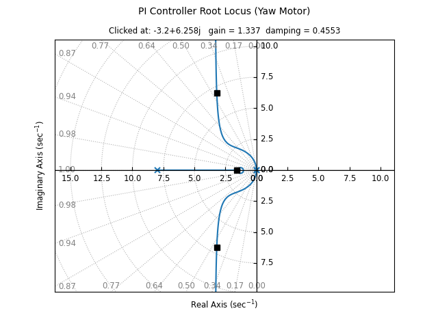
Figure 17: Yaw motor PI controller root locus

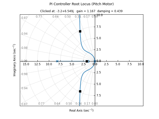
Figure 18: Pitch Motor PI Controller root locus

Figures 19 and 20 show the simulated step response of the yaw and pitch PI controllers for a 10-degree step input. While the settling time and zero steady-state error requirements were met, the percent overshoot exceeded the desired limits. This issue arises because the added zero ($z_{PI}$) is located too close to the origin, increasing the weight of the impulse response. This effect can be analyzed through the partial fraction expansion of $G_c(s)G_p(s)$. Although the extreme overshoot is not ideal, the primary focus remains on achieving the desired settling time and steady-state error.

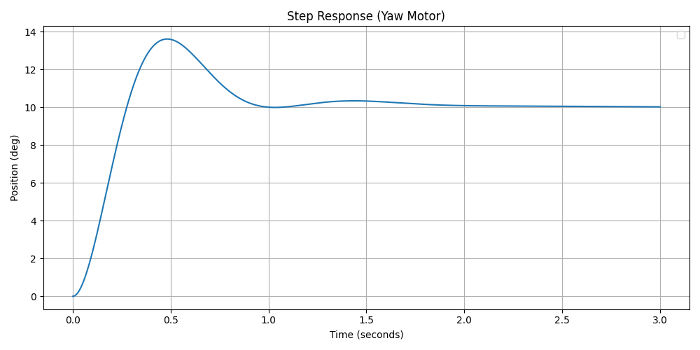
Figure 19: Simulated yaw motor PI control

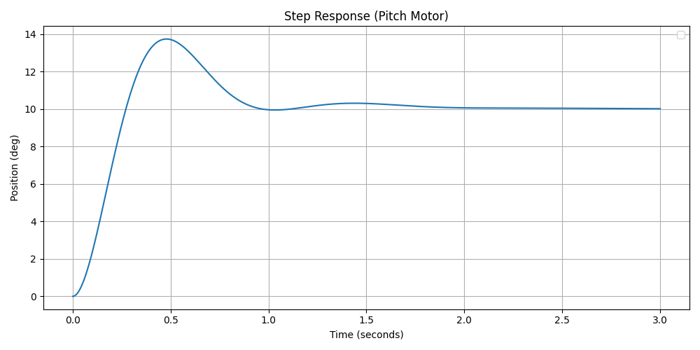
Figure 20: Simulated pitch motor PI control

The microcontroller operates in discrete time, processing sensor data in discrete snapshots rather than continuously. To convert the tuned continuous-time PI controller into a discrete-time controller, forward Euler approximation was used. While Tustin's approximation offers better frequency response matching with the continuous PI controller, forward Euler approximation was chosen for its simplicity. With a sampling rate of 60 Hz, the time interval between sensor measurements is small enough that the limitations of the Euler approximation are negligible, effectively making the controller behave as if it were continuous. This implementation is detailed in the controller.py script in the GitHub repo.

Figure 21 illustrates a functional diagram of the system with the PI controller implemented. The user, eventually replaced by a computer vision system, inputs a desired position in degrees for yaw and pitch. This desired position is sent to the PICO, where it is stored as the reference position. The PI controller uses this reference position to calculate the yaw and pitch errors and sends corresponding duty cycle commands to the motor controller. The motor controller, as previously discussed, regulates the voltage and drives the motors at the duty cycle specified by the Pico. As the motors move, their position is detected and measured by the IMU mounted on the turret. The IMU transmits its measurements to the Pico at a rate of 60 Hz, allowing the controller to continuously update the motor commands until the position error is approximately zero. This closed-loop feedback system enables the turret to move from its initial position to the desired position with accuracy and stability.

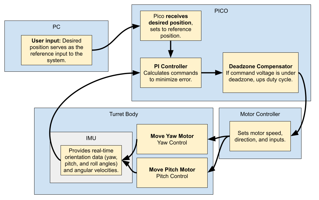
Figure 21: Functional block diagram describing the process of the PI controller

It is also important to note in implementation that the controller may theoretically order a voltage that is greater than the motor’s maximum 12V. To prevent that, the maximum duty cycle is limited to +/- 100%.

The gains calculated using the Root Locus method served as the initial starting point for tuning the actual turret motors. While the simulated response suggested reasonable settling times and zero steady-state error, real-world implementation revealed that these initial gains were suboptimal. The most significant issue was excessive overshoot, leading to prolonged oscillations and an extended settling time beyond the desired parameters. This discrepancy likely stemmed from the oversimplification and imperfections in the system’s estimated transfer function.

To refine the controller after the Root Locus analysis, $K_p$ and $K_i$ were incrementally adjusted. Initially, excessively high overshoot and oscillations indicated that $K_p$ was too large. After reducing $K_p$, $K_i$ was gradually increased until the controller achieved near-zero steady-state error. The final gain values were determined as follows: Yaw: $K_p=0.7$ $K_i=3.1$ Pitch: $K_p=0.8$ $K_i=3.2$.

The turret’s physical structure also introduced control challenges. The weight distribution affecting pitch control was not ideally balanced, as described in the System Modeling section. Additionally, because the IMU was not perfectly aligned to the turret’s center of rotation, yaw movements inadvertently affected the measured pitch, causing errors in the PI controller. To mitigate this, the control logic was modified to prioritize yaw adjustments before settling pitch control.

Performance Evaluation

The final implementation of the controller, shown in Figure 22, performed well for standard turret targeting within the camera’s field of view, requiring movements of up to 20° in yaw and 10° in pitch. In these cases, the turret consistently achieved a settling time between 1.24 and 1.50 seconds. However, the percent overshoot exceeded the desired 20%, reaching 57% for yaw and 51% for pitch. Despite this, the overshoot was deemed acceptable since the system still met the required time constraint to fire shots, which was the primary objective. The steady-state error measured 0.0625° for yaw and 0.4375° for pitch, slightly above the simulated zero error but within the ±1° accuracy requirement. Overall, these results met the problem statement and grading criteria.

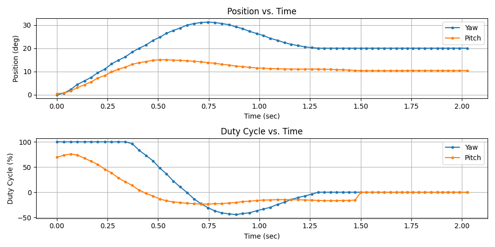
Figure 22: An “average use case” test of the PI controller

To verify the controller’s ability to rapidly shift between multiple targets, the turret was tested at its operational extremes, as shown in Figure 23. This test involved larger movements of 40° in yaw and 20° in pitch, exceeding typical use case requirements. While percent overshoot and steady-state error remained consistent with the standard tests, the settling time increased to 2.12 seconds for yaw and 2.41 seconds for pitch. This increase was primarily attributed to the time required for the motor to complete large deflections, even when operating at full speed, as indicated by the 100% duty cycle at the start of movement. Understanding these timing constraints provides valuable insight into the turret’s maximum response time for target acquisition.

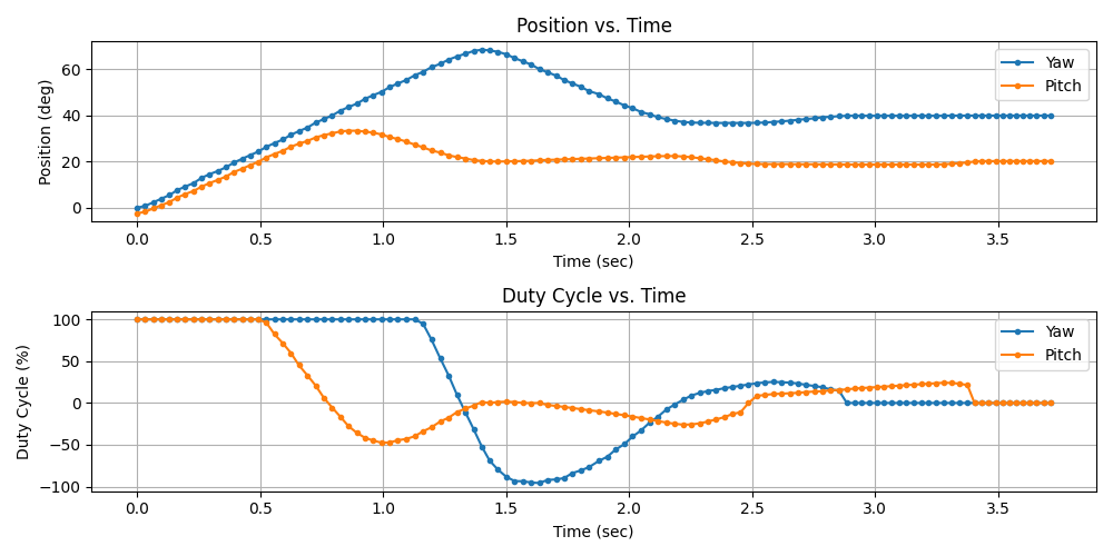
Figure 23: An “extreme” test of the PI controller

Firing Subsystem

The firing subsystem of the turret is responsible for controlling the motors that load and accelerate a desired number of balls toward the target, which includes a counter-rotating wheel motors, solenoid, and feed belt motor. To achieve this, MOSFETs are used as electronic switches to turn the components on and off. These transistors provide for a fast response time and increased reliability over other solutions such as relays. They also make it simpler to implement PWM due to its high switching frequency. However, that benefit was unnecessary for the firing subsystem as the motors and solenoid only need to be fully on or off if it is assumed that the counter rotating wheels are fully spun up when fired.

Fig. 24 illustrates the circuit used in the firing subsystem to provide a conceptual understanding of its design. All motors are actuated using N-channel MOSFETs, which allow the microcontroller to effectively control power even when the required current or voltage exceeds the capability of the Pico. A 10kΩ pull-down resistor is connected between the MOSFET gate and ground to prevent unintended switching in the absence of a control signal. Without the resistor, the gate could close, causing unintended motor actuation. A flyback diode, shown across the motor’s terminals, protects the circuit from high voltage spikes generated by the motor’s inductive load when switching on or off, safeguarding both the motor and the circuit.

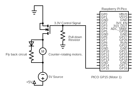
Figure 24: Firing system partial circuit diagram for conceptual understanding

As shown in the circuit diagram, the MOSFET’s drain connects to the motor’s negative terminal, while the source is grounded, with the flyback diode oriented in reverse polarity to the power supply to effectively block voltage spikes. This configuration ensures a stable, efficient firing mechanism, reducing the risk of motor failure and protecting electronic components from damage. This configuration is simplified in Fig. 24 to show only the counter rotating motors’ circuit; however, this design is used for every motor or potential inductive load in the firing system.

Fig. 25 is an image of the PCB with each of the important components of the circuit in Fig. 24 labeled. It is important to note that both the solenoid and feed belt motor operate at 12V and the firing motors operate at 5V.

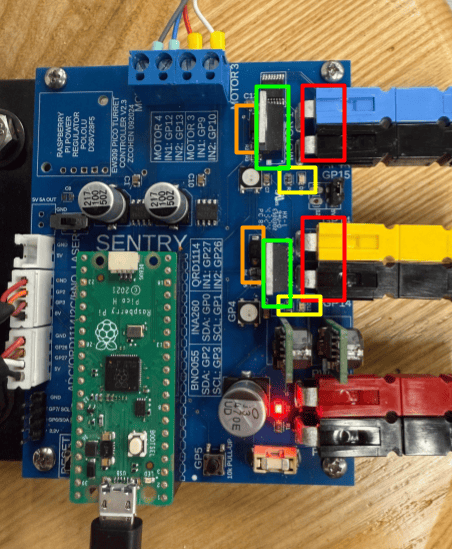
Figure 25: Turret printed circuit board with labeled components—Pull down resistors (orange), Fly back circuit (yellow), MOSFET (green), and Voltage source (red)

The first step in firing a ball is to ensure that the counter-rotating wheels are spun up to full speed to prevent the balls from getting stuck. This can be achieved using the INA-260 current sensor to measure the current through the 5V DC motors. If the measured current is above 0 amps, the motor can be determined to be powered on. However, it’s important to account for the spin-up time of the motor.

At startup, the current draw is initially high due to the low back EMF caused by slow motor speeds. As the motor speeds up, the back EMF increases, which reduces the current draw. Therefore, if the measured current drops below about 2 amps, the motor can be considered fully spun up.

Once the wheels reach operational speed, the 12V DC solenoid and feed belt motor are switched on to begin pushing the balls into the shooting mechanism. Shots can be detected by large spikes in the current through the 5V DC motors, which signify an increase in torque caused by the balls being pushed into and out of the wheels.

When utilizing this shot detection method in code, the PICO calculates the slope between each current measurement. If the slope exceeds a threshold of 20 A/s, a shot is counted. When firing multiple balls, the feed belt remains powered until the desired number of shots is counted. The code implementation is detailed in the GitHub repo.

Fig. 26 presents the measured current while firing five balls, highlighting the current spikes that correspond to each shot. The first spike is ignored by the PICO, as it results from the initial transition from not reading current at zero amps to reading current at about one amp during start up. By using this method, it is possible to monitor and ensure consistent and reliable performance.

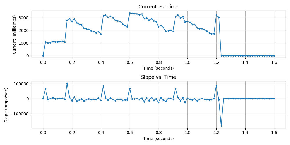
Figure 26: Current vs. Time and Slope vs. Time Plots

Fig. 27 illustrates the full process from the user making commands to the system firing. When the user orders a number of shots to be fired, the Pico spins up the firing motors, then loads balls and shoots for the number of shots requested. To keep track of the balls fired, the Pico monitors current spikes and records a shot when the current spikes dramatically indicate a ball was loaded. Importantly, the solenoid and the feed belt motor actuate together.

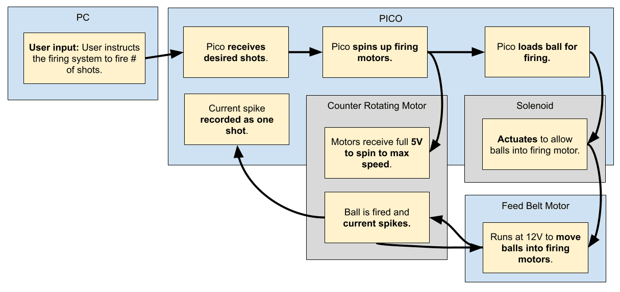
Figure 27: Firing subsystem functional block diagram

There were some complications in implementing the firing system. First and most critically, a maximum of eleven balls may be placed in the feed system, with one required to occupy the front most ammo slot while the remaining balls are loaded into the rear two slots. If this configuration is not followed, the gun either jams or fails to feed the ammunition properly down the belt. Additionally, it was observed that allowing the counter-rotating firing motors to spin up completely before launching a projectile was essential. Failing to do so resulted in the projectile either jamming in the system or rolling out of the barrel with minimal force.

During testing, inconsistencies in the firing sequence were encountered in which only two balls were fired instead of the desired three. This had to do with the way in which the system monitored balls shot and the initial spike of current to spin up the motor being counted as a fired shot, thus resulting in one less shot than requested. On the contrary, when the gun was angled downward, allowing gravity to push the balls into the counter-rotating wheels, the balls shot out too quickly for the PICO to register consistent current fluctuations. Because the current spikes didn’t always peak at the same level and sometimes didn’t drop significantly before the next spike, using a fixed current threshold became impractical. This necessitated the implementation of the slope method which proved to be more consistent at counting balls.

Computer Vision

The computer vision subsystem is responsible for identifying and classifying valid targets, and communicating those targets’ coordinates to the turret for engagement. The final implementation used the Luxonis OAK-1 Lite camera for image acquisition and YOLOv11-based object detection. This section explains the system setup, the training process, model evaluation, and implementation details to support reproducibility.

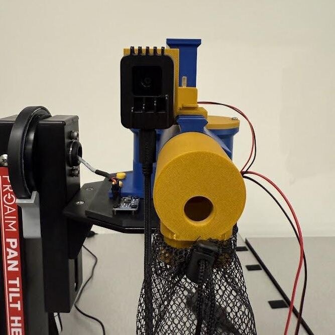
Figure 28: Sentry turret displaying the offset mounting of the OAK camera

As shown in Fig. 28, the camera is rigidly mounted above the Sentry turret, oriented to face forward and aligned closely with the turret's muzzle. The camera receives power and transmits data via a single USB-C connection to the host laptop, which runs the computer vision. The image frame and muzzle axis are not perfectly aligned, but calibration was performed to account for this offset. Before any target can be detected, the system must first capture an image that the model can process. This begins when the OAK-1 Lite camera captures a single frame and sends it to the host laptop over USB. The DepthAI API provides access to the video stream, enabling interaction with the camera's output. The video stream was configured to 1080p resolution at 30 frames per second, as detailed in Appendix A. Using the getCvFrame() method, this stream is converted into a standard OpenCV image. Once the image is received on the PC, it is passed into the YOLOv11 object detection model. This process ensures that each cycle starts with a fresh, real-time image of the turret’s field of view. A more complete process can be seen in the functional block diagram, Fig. 29, and is illustrated in the GitHub repo.

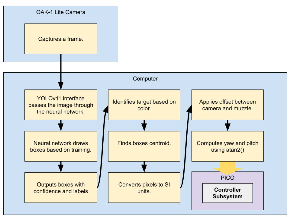
Figure 29: Computer vision subsystem functional block diagram

Target detection was performed using a trained Deep Neural Network (DNN) using the YOLOv11 architecture. The YOLOv11 small model was selected as it offers a balance between both speed, using a laptop CPU, and accuracy of the target detection. A larger model would result in a more accurate detection but would require more computing power which is limited. Should a discrete graphics card be implemented, a larger model can be utilized.

The training process began with collecting images of the target board with multiple colors and sizes of circles and different lighting conditions using the OAK-1 Lite camera. A total of 20 images were collected to include 4 images of just the background to improve the robustness of the model from false positives. Then, each image was labeled using the AnyLabeling annotation tool and formatted using the YoloDataPrep.py script. This data script outputs the required file structure, splitting the data into train and validate sets (80% train and 20% validate), converting all images into 640x640 pixels, and creating a data.yaml file for training with the Ultralytics YOLO framework. Initial training was performed on a GPU laptop using the YoloTrainGPU.py script with 100 epochs.

To further increase the effective size of our dataset and improve the network, image augmentation was performed by running the YoloAugment.py script. This included random cropping and brightness adjustment. These augmentations allowed the model to learn under a broader set of visual conditions, improving robustness to lighting changes and target occlusion. This process effectively tripled the size of the dataset for a total of 60 images (48 train and 12 validate). Using the trained weights from the original dataset, the YOLOv11 model was trained for an additional 100 epochs including the augmented images.

The trained model outputs bounding boxes with class labels and confidence scores for all detections. Valid detections were filtered using confidence, how much faith the model has in its prediction, and intersection of union, a measurement of how well the predicted bounding box overlaps with the true bounding box. The yolo.py script handles runtime inference on the laptop, and the model was evaluated using several performance metrics. All code can be found in the GitHub repo.

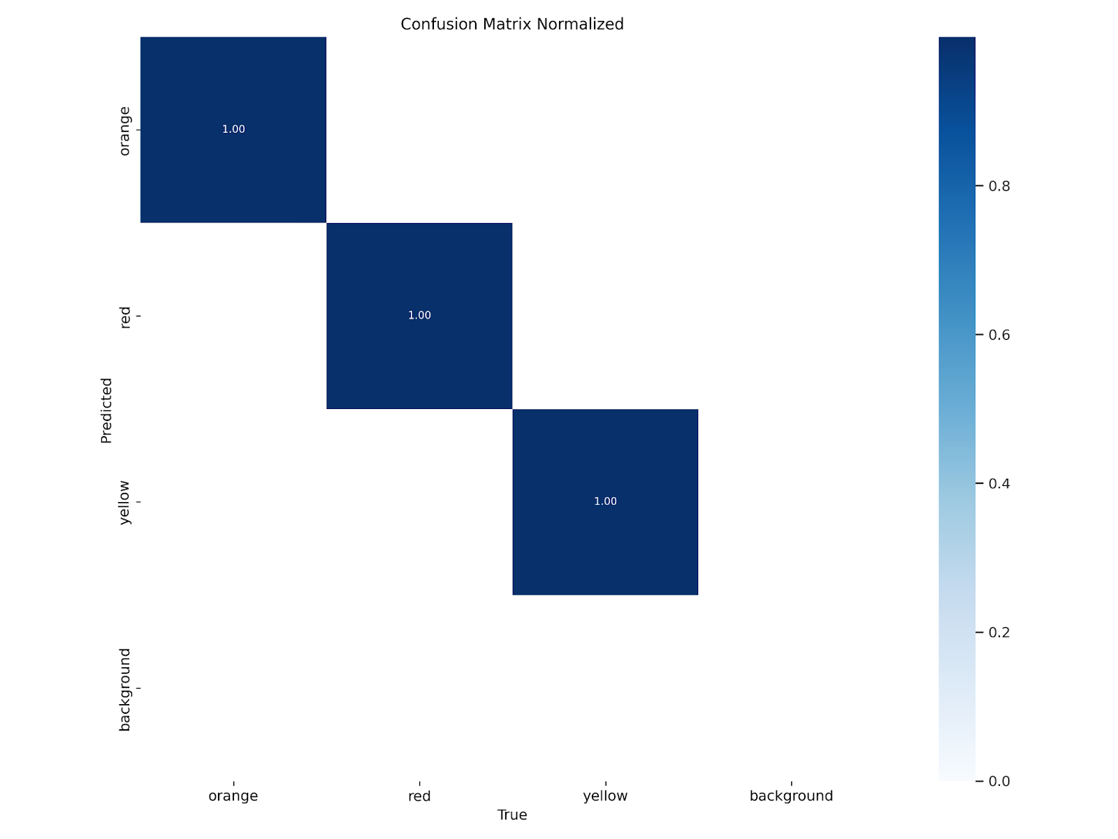
Figure 30: Normalized confusion matrix displaying perfect DNN performance

The normalized confusion matrix, in Fig. 30, illustrates perfect classification performance across all three target classes: orange, red, and yellow. There were no false positives or misclassifications. It is important to note that background is not treated as a class in YOLO, so the absence of a "background" row or column in the matrix is expected. The confusion matrix also demonstrates that no background regions were incorrectly classified as a target, which is ideal.

Figure 31: Precision-Confidence curve that details precision based on the model’s confidence level

The precision-confidence curve, in Fig. 31, illustrates how all target classes achieved precision close to 1.00 (perfect) at confidence thresholds above 0.95. This indicates that the model maintains high precision as confidence increases. The curve for the combined classes shows perfect precision at 0.971 confidence.

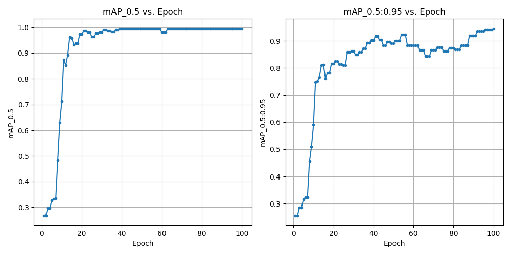
Figure 32: Original dataset training mAP

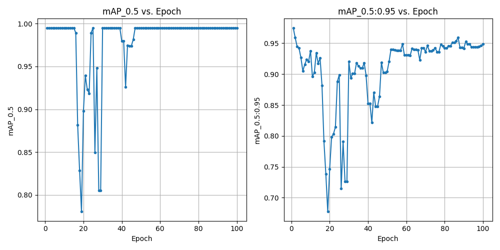
Figure 33: Augmented dataset training mAP

The mAP (mean Average Precision) plots from the training runs show that both models rapidly achieved high performance. Fig. 32 represents training with the original, unmodified dataset, while Fig. 33 displays results after augmenting the dataset. In both cases, the mAP@0.5 reached nearly 1.00 at 30 epochs, while mAP@0.5:0.95 continued to improve, ultimately surpassing 0.92. The mAP@0.5:0.95 offers a stricter evaluation metric of the model’s performance and explains why it was trained to 100 epochs.

The detected target sizes can be measured by counting the height of each bounding box and converting the number of pixels to SI units via,

$\text{Height}_{\text{SI}}=\frac{\text{Height}_\text{Pixels}*Z}{f_y},$

(22)

where $Z$ is the distance from the camera to the target and $f_y$ is the y-axis focal length. Should the bounding box have the correct height and class label as the specified target diameter and color, then that is the selected target. The vertical height was chosen to detect the target's diameter over horizontal width because the height is less likely to get distorted based on viewing angle.

Once a target is identified, the detection bounding box is used to calculate pixel coordinates of the target's centroid. Using the intrinsic parameters of the OAK camera and the pinhole camera model, the pixel to SI unit conversion can be calculated for x-axis pixels using,

$X=\frac{(u-c_x)Z}{f_x},$

(23)

and,

$Y=\frac{(v-c_y)Z}{f_y},$

(24)

for y-axis pixels. These equations use $(u,v)$ as the pixel coordinates, $(c_x,c_y)$ as the image output center, $f_x$ & $f_y$ as the focal lengths in pixels, and $Z$ as the distance from the camera to the image frame.

The converted pixel coordinates were then adjusted for the offset between the camera and turret muzzle before converting into yaw,

$\varphi=\varphi_0 + \left(\frac{x_{\text{adjusted}}}{Z}\right),$

(25)

and pitch,

$\theta=\theta_0 + \left(\frac{y_{\text{adjusted}}}{Z}\right).$

(26)

Here, $x_{\text{adjusted}}$ and $y_{\text{adjusted}}$ are the SI unit distance values from the camera’s center crosshairs to the selected target’s centroid and adjusted for ballistics bias. The angles $\varphi_0$ and $\theta_0$ are initial yaw and pitch angles of the gun, measured from the IMU during calculation. The calculated angles are then passed to the yaw and pitch controllers to aim the turret.

The model was validated by testing it against new images taken in different lighting conditions and with different backgrounds. During testing, some parameters were adjusted such as minimum area, eccentricity, and detection confidence threshold to reduce false positives and tune responsiveness. The model demonstrated consistent performance, effectively detecting and classifying objects with precision, even under challenging conditions such as sharp camera angles. Furthermore, camera pointing accuracy was tested using (23), (24), (25), and (26) without firing bias adjustments to estimate the required yaw and pitch angles for camera target acquisition. These angles were sent to the turret’s motor controllers, successfully positioning the camera’s crosshairs to align with the selected targets, within the error margin of the position controller.

Ballistics Testing and Analysis

The effectiveness of autonomous turret systems depends heavily on consistent accuracy and precision across the 10 to 20 feet range. To evaluate these characteristics, a statistical analysis of projectile impact patterns was conducted using a ballistic testing procedure at 10 ft, 15 ft, and 20ft as described in Appendix B. The measured and calculated bias, precision error, Circular Error Probable (CEP), and confidence intervals were used to determine the system’s targeting behavior. This report presents a comprehensive analysis of shot groupings, trends in system behavior over different distances, and the probability of hitting shots on target.

Testing Approach

To collect ballistics information on the SENTRY turret, several key concepts were applied to evaluate system performance in terms of accuracy and precision. The primary objective was to analyze shot dispersion at set distances of 10, 15, and 20 feet in order to characterize bias, the average deviation from the point of aim, and precision, the spread of shots around that average. The analysis was based on the assumption that shot impacts follow a Gaussian distribution, which enabled the use of Circular Error Probable (CEP) to assess overall targeting consistency.

The testing environment was structured to ensure consistent data collection. A chalkboard coated in white chalk provided a clear visual record of each impact point. A crosshair was drawn at the center of the board to serve as the point of aim. Since the turret lacks an internal homing system, the system was manually calibrated to align the turret’s camera view with the crosshair before each round of testing. At each distance, a total of 30 shots were fired to ensure sufficient sample size for a normal distribution. The x and y coordinates of each point of impact were measured relative to the crosshair using a yardstick with centimeter markings.

Data analysis included the calculation of mean impact location, standard deviation, and CEP both before and after applying bias correction. CEP diagrams were generated to visualize the likelihood of impacts falling within a defined radius around the point of aim. These diagrams and calculations were used to determine the minimum number of shots required to achieve a 95% probability of hitting a 5-inch diameter target, accounting for range dependent variation in accuracy and precision. The full experimental setup, procedures, schedule, and risk mitigation strategies are included in Appendix B.

Ballistics Data Analysis

A shot pattern analysis was conducted at three distances: 10 feet (304.8 cm), 15 feet (457.2 cm), and 20 feet (609.6 cm) to evaluate the accuracy and precision of the firing system. At each distance, 30 shots were taken and measured relative to the intended point of aim. Data was collected in a spreadsheet and imported to a Python script for statistical analysis and visualization.

The goal of the data analysis was to determine precision and bias. Bias is considered to be mean error in the horizontal and vertical directions, and precision is defined as the consistency of shot placements, measured by how tightly the impacts cluster around their average location, regardless of their proximity to the intended target. For each range, the x and y bias, the precision error, the 50% circular error probable (CEP), and the 95% confidence interval were calculated. CEP is given by,

$\text{CEP}_{50\%}=k*S_p,$

(27)

with the scale factor, $k=1.1774$, and the precision error, $S_p$ calculated using,

$S_p=\frac{1}{2}(S_x+S_y),$

(28)

where $S_x$ and $S_y$ are the standard deviations of the x and y impact locations.

The 95% confidence interval on the CEP can be calculated using,

$\sqrt{\frac{(n-1)S_p^2}{\chi_{(1-c)/2}^2}},$

(29)

for the lower-bound, and,

$\sqrt{\frac{(n-1)S_p^2}{\chi_{(1+c)/2}^2}},$

(30)

for the upper-bound where $n$ is the sample size (30 shots), $c$ is the confidence level (95%), and $\chi^2$ represents the Chi squared distribution.

The three trials at 10 feet (304.8 cm), 15 feet (457.2 cm), and 20 feet (609.6 cm) produced the results in Table 1.

Table 1: Ballistics Data

Target Range (cm)	x-bias (cm)	y-bias (cm)	Precision Error (cm)	Number of shots
304.8	-7.59	-26.08	3.41	30
457.2	-9.75	-46.03	5.78	30
609.6	-15.17	-74.35	7.26	30

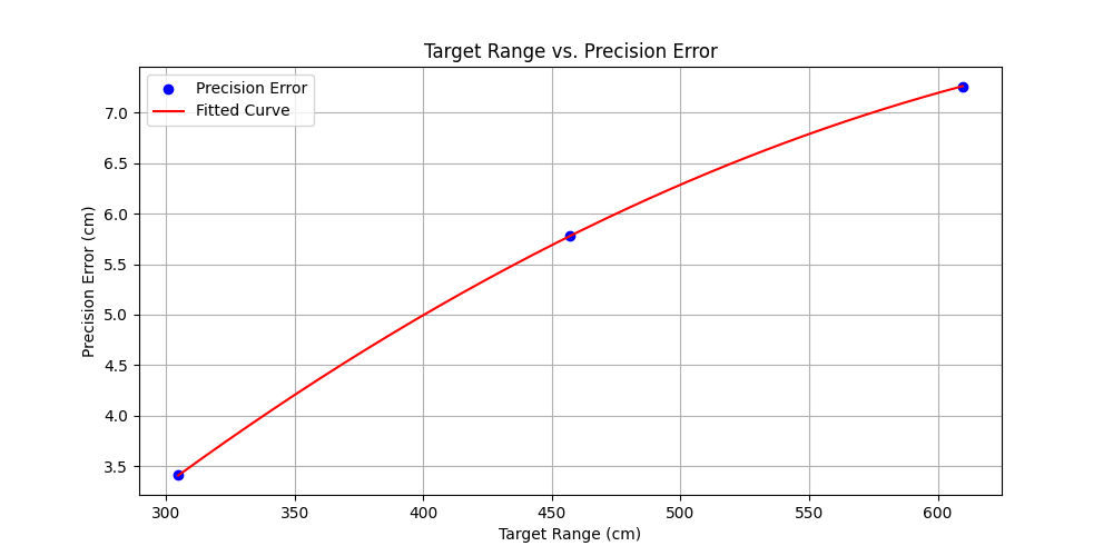
Figure 34: Target Range vs. Precision Error

Fig. 34 illustrates the relationship between target range and precision error. As shown, precision error increases with distance, indicating that shot groupings become less concentrated at longer ranges. The blue data points represent measured precision errors at three discrete distances: 10 feet (305 cm), 15 feet (457 cm), and 20 feet (610 cm). The red line represents the best fit to the data, achieved with a second-degree polynomial. This was the correct choice as the curve matches the data well.

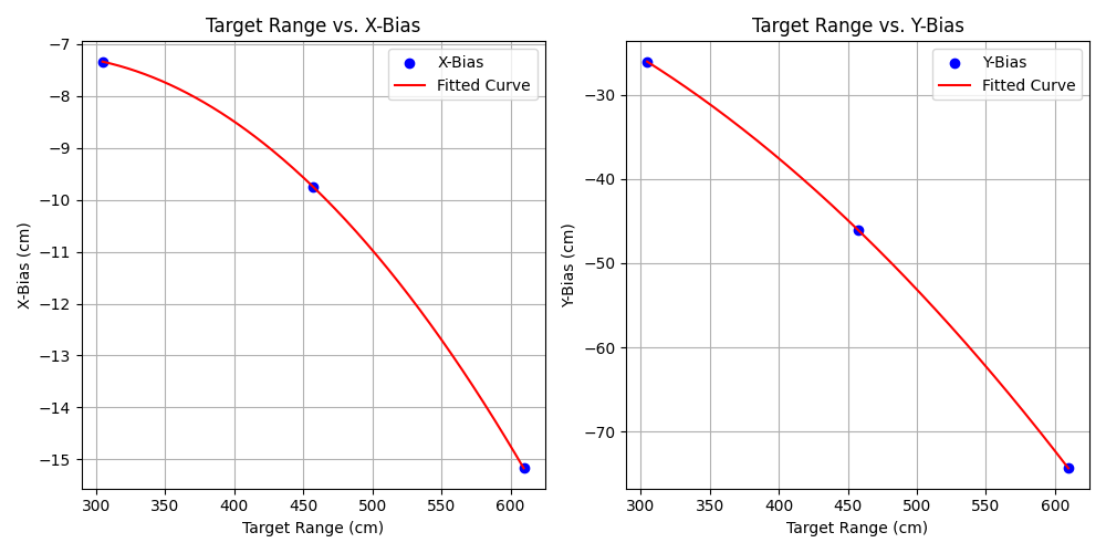
Figure 35: Target Range vs. X-Bias and Y-Bias

The plots in Fig. 35 display the x-bias and y-bias of the firing system as a function of target range, along with a fit line. The bias moves further down and to the left the further the turret is from the target. A bias down and to the left is expected because the camera is mounted up and to the right of the barrel, as shown previously in Fig. 28. It is also important to notice how the y-bias decreases rapidly with target range due to bullet drop. Both fitted curves closely follow the measured data points, suggesting that a quadratic model is appropriate for capturing the systematic deviations in both dimensions.

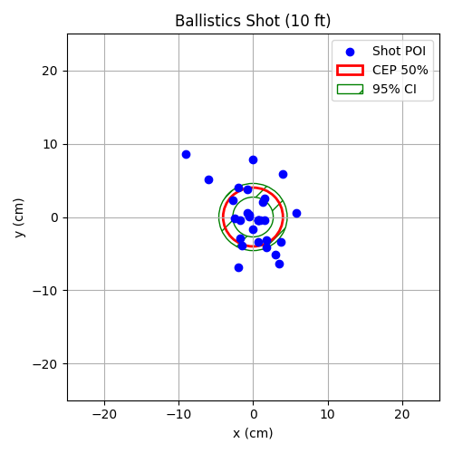
Figure 36: Shot Distribution at 10 ft (305 cm)

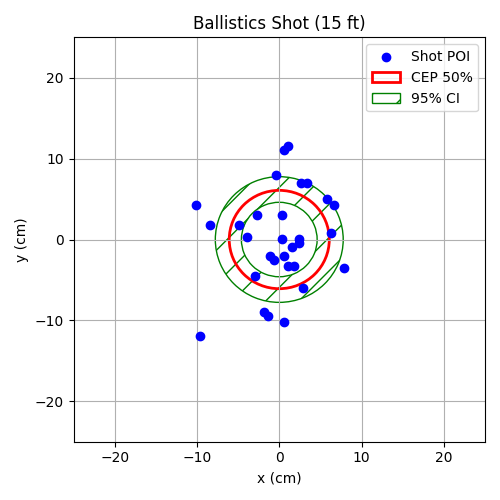
Figure 37: Shot Distribution at 15 ft (457 cm)

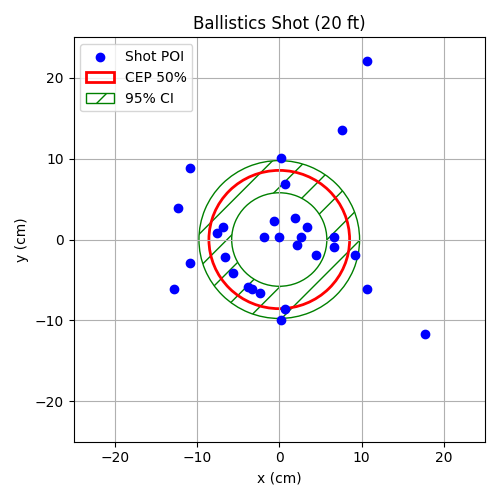
Figure 38: Shot Distribution at 20 ft (610 cm)

Fig. 36, Fig. 37, and Fig. 38 display the shot distributions at 10 ft, 15 ft, and 20 ft corrected for bias and each overlaid with the 50% CEP boundary and a 95% confidence interval ellipse. The CEP was calculated using the average of the standard deviations in the x and y directions and scaled by a constant factor $k=1.1774$, as in (22). As expected, CEP values increase with range, indicating that shot dispersion becomes more pronounced at greater distances.

In addition to the CEP, a 95% confidence interval was constructed around each shot grouping using (29) and (30). The confidence interval provides a visual representation of how well the CEP can be trusted. A thinner interval would suggest greater precision and reliability of the CEP, while a wider interval indicates more variability in the shot data and less certainty about the true precision of the firing system.

Given the x and y biases at several ranges, the polynomial curves in Fig. 35 can be used to estimate the correct bias distances at a given target range. Furthermore, the calculated precision error, $S_p$, allows for determining the minimum number of shots to achieve a 95% probability of hitting a 5-inch target at any specified range at least once. This is estimated by first calculating the scale factor,

$k=\frac{\text{CEP}}{S_p},$

(31)

where $\text{CEP}$ represents the radius of the 5-inch target, measured at 6.35 cm, and $S_p$ denotes the estimated precision error at a range of 10 to 20 feet, determined using the fitted curve in Fig. 34. With the scaling factor, the probability that the target is hit with only one shot, $p$, can be calculated with,

$p=1-e^{-\frac{1}{2}k^2}.$

(32)

The number of shots required for a 95% chance $(P_\text{one}=0.95)$ of at least one hit, $n$, can then be estimated using,

$n=\frac{\log(1-P_\text{one})}{\log(1-p)}.$

(33)

The code implementation can be seen in the GitHub repo.

The ballistics testing procedure revealed several challenges that informed both data collection and analysis. First, the target backdrop was initially positioned too low, causing several projectiles to strike below the measurement grid. This was corrected by raising the point of aim to capture all impacts within the chalk grid.

Second, a small number of errant shots appeared as statistical outliers and skewed the bias calculations. To mitigate this, the 15 ft dataset was re-measured in two additional trials, ensuring that bias corrections reflected the true systematic offset rather than anomalous points.

Finally, overlapping impact marks occasionally made individual shots indistinguishable. Breaking the 30-shot series into three subgroups of 10 shots each reduced overlap and improved the accuracy of impact localization. These adaptations improved the robustness of the computed x and y biases, the precision error $S_p$, and the resulting $\text{CEP}$ and 95% confidence regions.

System Integration

The system was designed from the outset with integration in mind. Each subsystem was modular, as illustrated in Fig. 39, yet structured to communicate via serial messages managed by the host PC. During integration, the most significant adjustments involved refining communication between the PICO and the PC. Initially, serial messages consisted of simple commands. However, as the vision, firing, and control systems were combined, the message structure was expanded to include targeting angles and shot counts. This allowed a single serial command to fully direct the turret, eliminating the need for multiple transmissions per action.

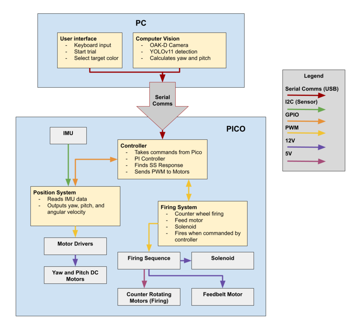
Figure 39: Full system block diagram

Each subsystem—vision, control, feedback, actuation, and firing—was first developed and tested independently before being bedded into the full system. This incremental approach made it easier to isolate bugs and ensured that core functionality was preserved as system complexity grew. The codebase was structured for flexibility, enabling features to be easily added or removed. For example, PICO scripts were built in layers, allowing them to operate even when certain components were disabled. This stratified approach enabled rapid testing and simplified troubleshooting when subsystems interfered.

One recurring issue during integration was finalizing the serial message format. Initially, each subsystem used its own custom string structure. As components were unified under a single control message, the format was standardized to convey all necessary data for the turret to hit its target. The final command format, “Target 1: Yaw angle, Pitch angle, Fire count, Target 2: Yaw angle, Pitch angle, Fire count”, required synchronized logic on both the laptop and PICO to interpret and execute properly.

Another integration challenge involved timing and command sequencing. If a new target was passed to the PICO while the turret was still aiming, it could interrupt the control loop mid-motion. To address this, commands were sent in complete blocks, enabling the PICO to operate autonomously through each shot sequence. Once a block was received, the PICO would execute the motion, assess when the turret had settled using the slope of error and position change, fire the designated number of shots, then move to the next target. This sequencing became essential when integrating vision, control, and firing systems.

Controller tuning required further refinement due to inconsistent steady-state error in the system’s response. The yaw and pitch controllers needed to handle both large (up to 40°) and small (as little as 5°) angular movements. Both of which extended beyond the scope of earlier testing. To resolve this, we revisited the process detailed in the Controller Design section and incorporated the Ziegler-Nichols tuning method to estimate appropriate initial gains. These were then iteratively adjusted through trial and error to provide a significant reduction in steady-state error while preserving acceptable overshoot and settling times. The final tuned gains were: Yaw: $K_p=1.44$ $K_i=6$ and Pitch: $K_p=1.44$ $K_i=6.24$. This tuning ensured precise and stable positioning, critical for reliable turret performance.

Memory constraints on the PICO also necessitated internal changes. Originally, the microcontroller stored the error at each loop iteration to aid in tuning and analysis. However, as demands grew (parsing incoming messages, driving motors, reading IMU data, and managing the firing system) this approach caused PICO memory overflows and system crashes. To address this, the on-board error logging was replaced with a lightweight steady-state detector using only the most recent error and its slope, significantly reducing memory usage and allowed the system to run continuously through multi-target scenarios.

Ultimately, the system came together through deliberate modular design and careful sequencing of operations. Integration surfaced several issues, such as message structuring and memory management, that were not apparent during isolated testing. Resolving these challenges not only strengthened the systems robustness but also provided a realistic sense of what it takes to engineer a fully working solution.

Results and Conclusions

This section presents the final evaluation of the autonomous turret system, detailing the demonstration procedures, system performance relative to the grading rubric, and key lessons learned throughout the design and integration process. The following subsections summarize the system’s performance during live trials, evaluate its ability to meet both engineering and operational requirements, and offer recommendations for future students developing similar autonomous platforms.

Final Demonstration Approach

The final demonstration was conducted in accordance with the EW309 scoring rubric and consisted of three trials. Each trial required the turret to autonomously detect and engage two 5-inch diameter targets of a specified color (10 to 20 feet from the gun), positioned at opposite corners of the chalkboard and surrounded by decoys of varying sizes and colors. The targets were placed both above and below the camera’s centerline, as well as to the left and right, maximizing the required angular movements between engagements. The turret was required to aim and fire at both targets within 15 seconds and 1-2 hits per target. The materials used during the final demo are outlined in Table 2, and the required settings/configuration for each trial are detailed in Table 3.

Table 2: Required final demo parts list

Part	Description
SENTRY Turret System	Prefabricated EW309 turret
Laptop	Runs computer vision and sends serial commands to the PICO
Raspberry Pi PICO	Microcontroller for motor control and sensor processing
OAK-1 Lite Camera	Provides real time video input to the laptop
5-inch Circular Targets	Instructor provided; red, yellow, and orange
Target Chalkboard	Large enough to mount targets in all quadrants
Power Supply (12V)	Powers motor drivers and firing subsystems
USB-C Cable	Provides power and data for the OAK-1 Lite camera
Micro-USB Cable	For serial communication and power between laptop and PICO
Projectiles (Nerf balls)	11 total (5 loaded per working column in the feed system and 1 extra balanced on top)

Table 3: Required final demo settings

Subsystem	Setting/Configuration
Camera Resolution	1080p at 30 fps
Camera Position	Mounted above turret muzzle, facing forward
YOLOv11 Model	Trained for orange, red, and yellow target colors
Target Detection	Set to specified color and target distance from camera
IMU Sampling Rate	60 Hz
Bias Offsets	Yaw/pitch bias adjusted for target range
Firing Motor Spin-Up	Begins before the targeting command for time optimization
Feed System Load	12 total balls with 5 in the back and middle column, on in the front column, and one stacked on top
Turret	Oriented to "zero" by aligning the muzzle to be perpendicular to the target board and the arm to mid-way between the two backstops

Each trial used a different designated target color. The YOLO-based computer vision model performed consistently well in all cases, successfully detecting targets regardless of the assigned color. The OAK-1 Lite camera streamed continuously from startup, using its default 1080p at 30 fps configuration. For each engagement, the PC used the vision model to track target positions and send a structured serial command to the PICO containing the computed yaw and pitch angles, along with the specified number of shots. Target prioritization was based on detection order. Since targets were placed at opposite ends of the board, the turret had to execute wide sweeps with fast settling to meet time constraints. To aid in accuracy, pitch bias offsets were manually adjusted to compensate for range-dependent drift, with final adjustments made during pre-demonstration calibration. At the end of each trial, both the turret yaw and pitch errors, measured shot count, time, and observed number of hits per target were recorded.

Performance Measures

Our system was evaluated according to the five performance categories outlined in the EW309 final demonstration rubric: target identification, trial time, steady-state error, number of shots fired, and total number of hits. The turret achieved a perfect score, 5 out of 5 in each category, during its second trial, meeting all specified requirements and validating the effectiveness of our integrated design. The following sections break down each evaluation criterion and the system’s corresponding performance.

The turret accurately identified both specified targets using a custom-trained YOLOv11 model, capable of detecting 5-inch red, yellow, and orange circles. Across all three trials, the model consistently detected exactly two valid targets per run, even when placed at opposite corners of the target board. No false positives were recorded, and bounding boxes were correctly aligned. The system successfully ignored decoys of varying sizes and colors, fulfilling the requirement to exclusively identify specified targets.

In terms of trial time, the system successfully completed both engagements within the 15-second requirement during all three trials. To minimize startup delays, the firing motors were pre-spun before the trials began, ensuring the engagement sequence initiated immediately upon receiving the serial command from the laptop. The ability to detect, aim, and fire at two targets within the time limit demonstrated the responsiveness of both the PI motor controllers and the firing mechanism.

The system also met the steady-state error requirement, with both the yaw and pitch axes consistently remaining within ±0.01 radians (approximately 0.57 degrees). This level of precision was achieved through real-time IMU feedback feeding into PI controllers. A slope-based convergence method determined when the system had stabilized, allowing it to proceed confidently to the firing stage. These values were monitored and confirmed via serial output from the PICO to the laptop during the live trials. Even during wide-angle transitions between targets, the error remained within the acceptable range, confirming the reliability of the control system.

Regarding the number of shots fired, the turret was commanded to launch five projectiles per target according to (34). Shot count was confirmed both programmatically, by detecting current spikes during firing, and by direct observation. The firing subsystem performed reliably, even at full-speed operation, with only the third trial reporting a misfire of four instead of five shots.

Quantitatively, the system's second trial represents the benchmark performance of our design. The turret successfully identified both valid targets with zero false positives, even with multiple decoys in view. The full engagement sequence, from the start of targeting to the final shot, was completed in 13.7 seconds. Steady-state error remained within ±0.57 degrees, with final yaw errors of approximately 0.218 degrees and 0.293 degrees for Targets 1 and 2, respectively, and pitch errors of approximately 0.293 degrees and -0.336 degrees. The system fired exactly five shots at each target, confirmed by both current measurements and observers. Of those ten total shots, the turret achieved one confirmed hit on both targets, meeting the minimum hit threshold for full credit.

Areas for improvement include more extensive ballistics data collection. In the first trial, the turret hit each target more than twice despite being commanded to fire only five shots, suggesting that the shot count derived from the CEP was overly conservative. Expanding the ballistics dataset would help produce a more representative sample of the projectile dispersion pattern, leading to a more accurate CEP calculation and, in turn, a more precise estimate of the number of shots required to achieve at least one hit per target. Additionally, the shot-counting mechanism based on current spike detection could be further refined. During the third trial, the turret appeared to fire fewer shots than commanded, an issue that had not been surfaced in earlier testing. This discrepancy underscores the value of thorough, repeated testing to reveal unexpected failures and system uncertainties not visible during initial development.

Discussion and Conclusion

The final performance of our autonomous turret system highlights the strengths of modular design, integrated control, and robust vision processing. Across three live trials, the system achieved full marks according to the EW309 final demonstration rubric, with the second trial standing out as the benchmark. This outcome was made possible through clearly defined subsystem roles and deliberate coordination during integration. The turret consistently identified targets with zero false positives, responded to commands with sub-second steady-state error, and executed precise firing sequences within the required time limit.

Several factors contributed to this strong performance. The PI controller operated reliably under varying loads, consistently settling within the ±0.01 radian accuracy requirement. The vision system, powered by a YOLOv11 model, maintained high-confidence classification, even in the presence of multiple decoys. The streamlined serial communication protocol allowed the PC to transmit yaw, pitch, and shot count data in a compact format, enabling fast, reliable transitions between perception, control, and actuation. These design decisions allowed the turret to operate autonomously and reliably, without user intervention during each trial.

Despite this success, several limitations emerged. Mechanical inconsistencies in the hardware led to projectile drift, particularly at longer ranges. Even when fired directly at the target, shots displayed a noticeable downward bias due to the camera’s offset and gravitational effects. While pitch bias corrections partially mitigated this, they were not completely adaptive to changing conditions and required some adjusting. Mechanical jams and occasional current fluctuations also caused misfires that were difficult to detect preemptively. Additionally, the system required precise setup before each run, including ball loading, bias calibration, and manual shot count verification. Although these factors did not prevent the system from achieving full credit, they highlighted areas for improved robustness and reliability.

Based on our experience, we recommend several practices for future midshipmen working on similar autonomous systems. First, prioritize integration from the start. While individual subsystems may perform well in isolation, full integration reveals hidden timing issues, memory constraints, and unexpected interdependencies. Second, minimize onboard data logging and favor real-time analysis. Our initial design stored full error histories, which worked during testing but led to memory overflows in full demonstration trials. Replacing this with a slope-based convergence method resolved the issue. Third, don't underestimate hardware quirks. Testing ballistics thoroughly provides the data required to implement effective bias compensation. Lastly, implement live telemetry where possible. Sending real-time pitch/yaw error and shot count data back to the PC proved invaluable for analyzing system behavior and ensuring rubric metrics were met during live demonstrations.

In summary, this project successfully met all engineering objectives, delivering a fully autonomous turret capable of reliable, accurate real-time engagement. While setbacks in both hardware and software presented challenges, each one deepened our understanding of system integration and ultimately strengthened the final design.

References

[1] H. Shack. “Raspberry Pi Motion Tracking Gun Turret.” Hackster.io Accessed: Jan. 11, 2025. [Online]. Available: https://www.hackster.io/hackershack/raspberry-pi-motion-tracking-gun-turret-77fb0b

[2] C. Bermhed and J. Holst, "Design and Construction of an Autonomous Sentry Turret Utilizing Computer Vision," June 2023.

[3] T. Yathavi, "Development of Auto Tracking and Target Fixing Gun Using Machine Vision," presented at the 2020 ISCAN, Pondicherry, India, July 3-4, 2020.

[4] F. Yu and X. Zhao. "Autonomous Object Tracking Turret." Cornell Electrical and Computer Engineering. Accessed: Jan. 11 2025. [Online]. Available: https://courses.ece.cornell.edu/ece5990/ECE5725_Spring2018_Projects/fy57_xz522_AutoTurret

[5] M. Ahmed. “Improved PID Controller for DC Motor Control,” presented at the 2021 IOP Conf. Ser.: Mater. Sci. Eng., United Kingdom, 2021.

[6] Proaim "Proaim Sr. Pan Tilt Head for Camera Jib Crane." Proaim. Accessed: Jan. 21 2025 [Online]. Available: https://www.proaim.com/products/proaim-sr-pan-tilt-head-with-12v-joystick-control

[7] ROHM Semiconductor. BD62120AEFJ Datasheet. (2022). Accessed: Jan. 31, 2025. [Online] Available: https://fscdn.rohm.com/en/products/databook/datasheet/ic/motor/dc/bd62120aefj-e.pdf

[8] Raspberry Pi. RP2040 Datasheet. (2024). Accessed: Jan. 31, 2025. [Online] Available: https://datasheets.raspberrypi.com/rp2040/rp2040-datasheet.pdf

[9] keyboard. (2020). BoppreH. Accessed: Jan. 31, 2025. [Online] Available: https://github.com/boppreh/keyboard

[10] Bosch Sensortec. BNO055 Datasheet. (2014). Accessed: Feb. 9, 2025. [Online] Available: https://cdn-shop.adafruit.com/datasheets/BST_BNO055_DS000_12.pdf

[11] Adafruit_BNO055. (2024). Adafruit. Accessed: Feb. 4, 2025. [Online]. Available: https://github.com/adafruit/Adafruit_BNO055

[12] Micropython. (2025) Micropython. Accessed: Feb. 4, 2025. [Online]. Available: https://github.com/micropython/micropython

[13] Matplotlib. (2025) Matplotlib. Accessed: Feb. 4, 2025. [Online]. Available: https://github.com/matplotlib/matplotlib

[14] A. M. Mao, J. L. Moore, and L. L. Whitcomb, “Adaptive Identification of Second-Order Mechanical Systems with Nullspace Parameter Structure: Stability and Parameter Convergence,” presented at the 2024 IEEE 63rd CDC, Milan, Italy, Dec. 16-19, 2024.

[15] NumPy. (2025) Numpy. Accessed: Feb. 11, 2025. [Online]. Available: https://github.com/numpy/numpy

[16] Luxonis. OAK-1 Lite Datasheet. (2024). Accessed: Mar. 27, 2025 [Online]. Available: https://github.com/luxonis/depthai-hardware/blob/master/NG9096_OAK-1-Lite/Datasheet/OAK-1-Lite_Datasheet.pdf

[17] Raspberry Pi. Raspberry Pi Camera Module 3 Datasheet. (2024). Accessed: Mar. 27, 2025. [Online]. Available: https://datasheets.raspberrypi.com/camera/camera-module-3-product-brief.pdf

[18] Intel. Intel RealSense Product Family D400 Series Datasheet. (2020). Accessed: Mar. 27, 2025. [Online]. Available: https://www.intelrealsense.com/wp-content/uploads/2020/06/Intel-RealSense-D400-Series-Datasheet-June-2020.pdf

[19] D. W. Webb, “Circular Probable Error for Circular and Noncircular Gaussian Impacts,” U.S. Army Res. Lab, Aberdeen, MD, USA, ARL-MR-830. Accessed: Apr. 3, 2025. [Online]. Available: https://apps.dtic.mil/sti/pdfs/AD1043284.pdf

Appendix A: Error Analysis and Component Selection

Understanding System Errors

The SENTRY turret system is vulnerable to three major errors, including camera target tracking errors, IMU turret angle estimation errors, and controller tracking errors. Combining these systems together results in errors as well. If the camera and IMU sensors are not calibrated/aligned with each other, the system would be unable to point the muzzle accurately at the target.

At 10 feet, the turret must maintain a total system pointing error within ±1.22°, and within ±0.61° at 20ft. This demonstrates that the 20-foot range is the most demanding and is the “design driving distance.” Given that accuracy is the most important design criterion, the components must be selected and tuned to meet these requirements.

Camera tracking errors stem from difficulties identifying and targeting, or drawing a border around, the targets in each image. These errors may be caused by motion blur, poor lighting, limited resolution, or faulty coding. These issues may affect accuracy, how close the detected target is to actual location, and precision, any measurement noise. The system will quantify these errors by comparing images of the detected shot, where the ball is in that image, and its deviation from the center of the target over multiple trials.

Using the IMU to estimate the turret’s orientation introduces a source of potential errors. The BNO055 IMU uses its accelerometer, gyroscope, and magnetometer to estimate the pose of the turret. Using all of this data from multiple measurement sources improves the accuracy of the estimated orientation. Nevertheless, it is still sensitive to sensor drift and magnetic interference. Orientation errors from the IMU are measured by the manufacturer and provided as ± 1° for roll and pitch under ideal conditions [10].

Controller tracking error comes in the form of steady state error and the characteristics of the controller’s transient response, like settling time and overshoot. When it comes to target accuracy, steady state error is the most significant factor. Assuming the target fires upon reaching steady state, the settling time and overshoot primarily affects timing rather than accuracy. The controller’s steady state error was optimized to be less than ± 0.61°, with a maximum of 0.4375°. Theoretically, this should allow the turret to accurately hit a target at about 27 ft away.

To assess the impact of both IMU and controller errors on the turret’s accuracy, it is essential to analyze how each subsystem contributes to the overall error. While the controller meets the ± 0.61° error requirement, the IMU’s sensor accuracy poses a significant restraint. The IMU’s ± 1° error is unacceptable for the target at further ranges. Only at 10ft is the maximum permissible error ± 1.22°. Given the IMU cannot reliably meet the required accuracy specifications, it becomes a limited factor of the system’s overall performance.

There is also the potential for magnetic interference to degrade the IMU’s performance. Nearby electronics, metal, and other materials can disrupt the magnetometer and increase sensor drift. This issue is primarily mitigated by fusing gyro, accelerometer, and magnetometer measurements to estimate orientation. Fortunately, the issue of magnetic interference has not been a problem in preliminary testing. If it does become a problem, the fix would be to swap the IMU for a more accurate and robust sensor. However, given that the target is relatively close to the turret and stationary, magnetic interference should unlikely pose a significant challenge.

Camera Specifications

In researching necessary specifications for the camera used in the turret system, three machine vision cameras were discussed. The Luxonis OAK-1 Lite, the Raspberry Pi Camera Module and the Intel RealSense D455 camera specifications are listed in Table 4.

Table 4: Machine Vision Cameras

Specification	Luxonis OAK-1 Lite	Raspberry Pi Camera Module	Intel RealSense D455
Maximum Resolution	4056 × 3040 pixels	4056 × 3040 pixels	1280 × 800 pixels
Field of View (Horizontal)	81°	76°	90°

Among the three machine vision cameras evaluated, the Luxonis OAK-1 Lite is the most suitable for the turret system. It uses a 12 MP sensor with a wide 81° horizontal field of view [16]. The Raspberry Pi camera module is another good option because of its comparable resolution, but it is built specifically for Raspberry Pi microcomputers using an FPC connector which is incompatible with the laptop [17]. Alternatively, the Intel RealSense D455 features a wider horizontal field of view than the OAK-1 Lite. However, it’s designed for depth mapping and includes a dual camera stereoscopic system, which is not required for the turret’s application and adds extra costs [18]. The OAK-1 Lite provides a balance of resolution, field of view, and affordability, making it a suitable camera for the turret application.

The selected Luxonis OAK-1 Lite camera features a horizontal field of view (FOV) of 81° and a resolution of 4056×3040 pixels which gets cropped to 4k video output. While this high resolution will result in a larger pixel count and thus a more accurate target centroid estimation, it would lead to unnecessary high processing costs. As a result of this trade off, a resolution of 1080p or 1920x1080 pixels was selected. At 20 feet (6.1 m), the camera’s FOV corresponds to a scene width of approximately 10.42 meters via,

$\text{Scene Width}=2*Z*\tan{\left(\frac{\theta}{2}\right)},$

(34)

where $Z$ is the distance from the target and $\theta$ is the FOV. Given the horizontal pixel count of 1920, each pixel spans around 5.43 millimeters. This was calculated using,

$\text{Pixel Width}=\frac{\text{Scene Width (m)}}{\text{\# of Horizontal Pixels}}.$

(35)

A 0.13-meter (5-in) diameter target would therefore occupy about 24 pixels across at the 20 ft distance. This pixel count is sufficient for reliable centroid detection and targeting. This scene is illustrated in Fig. 30.

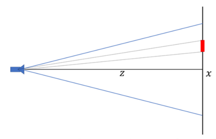
Figure 40: Geometry of Camera and Targeting (top view)

Camera-IMU Calibration

Aligning the camera and the IMU frames can help reduce systematic error. This calibration ensures that when the camera detects a target at some direction, the turret can rotate to the correct angle in the IMU reference frame. Calibration is performed by placing a known target at multiple angular positions across the field of view, recording both camera and IMU measurements, and solving for a transformation matrix between the two frames using least-squares. Calibration error must be kept low as small misalignments can cause consistent misses, especially at 20ft.

To diagnose calibration issues, the system will be tested at 10 and 20 feet, using known turret angles and target positions. If the turret consistently misses with minimal controller error, calibration is likely the root cause. To confirm this, the computer code will collect data and plot the camera’s detected target angle against the IMU’s reported yaw and pitch angles. Ideally, the plots should align perfectly, with any offset indicating a calibration issue.

Appendix B: Ballistics Testing Plan

The objective of this test is to evaluate the bias and precision of the SENTRY turret by analyzing shot dispersion at distances between 10 and 20 feet. It will serve to develop a targeting system that can deliver consistent shots at targets with a 95% hit probability. By understanding the gun’s bias and precision errors, we can implement corrections and determine the number of shots necessary for effective target engagement.

Testing Approach

For this test, the following is required:

1. SENTRY turret system.
2. SENTRY Python software suite (found in GitHub repo).
3. Computer.
4. Computer vision system.
5. Chalkboard backdrop.
6. White chalk (for impact marks).
7. Ruler or yardstick.
8. Measuring tape.
9. Safety eyewear.

The test will focus on bias and precision. Bias will test the shot’s deviation from the target and precision will test how tightly the shots cluster together.

To begin testing, position the SENTRY turret at a known distance from the target with the chalkboard fully in view of the camera, starting at 10 feet. It would be ideal to position the target at the same level as the chalkboard to avoid significant pitch tilt, which could affect the ballistic trajectory. Cover a 2x2 ft area of chalkboard in white chalk to clearly mark each point of impact (POI).

Calibrate the system to ensure the turret consistently aims at a defined target, such as the center of the chalkboard. This can be done by marking a crosshair on the chalkboard and manually aligning the camera feed’s crosshair with the chalkboard’s crosshair.

At each distance, fire a minimum of 30 shots to gather statistically reliable data representing a Gaussian distribution (Circular Error Probable assumes a Gaussian distribution). For each shot, record the x and y coordinates of the POI relative to the center crosshair using a ruler or yardstick. Collecting data for all 30 shots may be difficult due to overlapping impact marks, so recording data every 5–10 shots might be more practical.

Repeat this process at 15 feet and 20 feet. Collecting data at three ranges between the 10 to 20 feet interval is sufficient to provide insight whether the bias and precision errors follow a linear or nonlinear relationship.

After testing at all three distances, convert all x and y coordinates to SI units. Use this data to compute the mean (representing systematic bias), the standard deviation (representing precision), and the Circular Error Probable (CEP) after correcting for any bias [19].

A test is considered successful if each distance yields at least 30 shot data points, providing a sufficient sample size for analysis. The system must produce clear and measurable shot patterns at all tested ranges, allowing for meaningful evaluation of performance. Additionally, the data must support the calculation of the CEP, with at least 50% of the shots falling within the defined radius centered on the point of aim. Finally, the test must generate enough information to determine range dependent bias corrections (between 10 and 20 ft) and calculate the minimum number of shots required to achieve a 95% probability of hitting a 5-inch diameter target at a given range.

The deliverables from this test will include a comprehensive data table containing all x and y impact points converted to SI units. For each tested range, the calculated bias and precision errors will be presented, along with corresponding CEP diagrams after bias correction. A firing system will be developed to determine the number of shots required to achieve a 95% probability of hitting a 5-inch diameter target at 10 to 20 ft away.

Environmental Considerations, Test Schedule, and Risk Management

The test requires a safe indoor firing range which will be the EW309 classroom. A chalkboard will be used to capture the points of impact. The test can be effectively conducted with a team of two members: one responsible for operating the turret and conducting the shots, and the other focused on documenting the process, taking measurements, and managing image capture and analysis. Clear communication and coordination between the team members will be essential for accurate data collection and efficient execution.

The test schedule is illustrated in Table 5.

Table 5: Ballistics test schedule

Activity	Estimated Duration
Setup and calibration	30 minutes
Testing at 3 ranges (10, 15, 20 ft)	1 hour
Initial cleanup and data collection	30 minutes
Total Test Duration	~ 2 hours
Data analysis (post-testing)	~ 2 hours (depending on tools)

To ensure a smooth and reliable testing process, it is important to identify potential risks and outline strategies to mitigate them. Table 6 highlights key risks associated with the ballistics test and the corresponding actions that can be taken to minimize their impact.

Table 6: Ballistics test risk management

Risk	Mitigation
Misfire or hardware failure	Inspect turret before firing, press shutoff safety switch, and have backup cables/tools ready.
Inaccurate measurement	Use consistent units, double-check conversions, and use software tools when possible.
Safety hazard	Ensure turret only fires in a secure and cleared direction with safety glasses.
Inconsistent aim	Recalibrate aim at each distance using camera alignment method or a laser pointer.