Roomba Light Show

December 2025

GitHub Repository

Introduction

My seventh major course at USNA was EW456 (Autonomous Vehicles). The course focused on the kinematics, dynamics, and control of ground and aerial vehicles, utilizing both software simulation and experimental hardware validation.

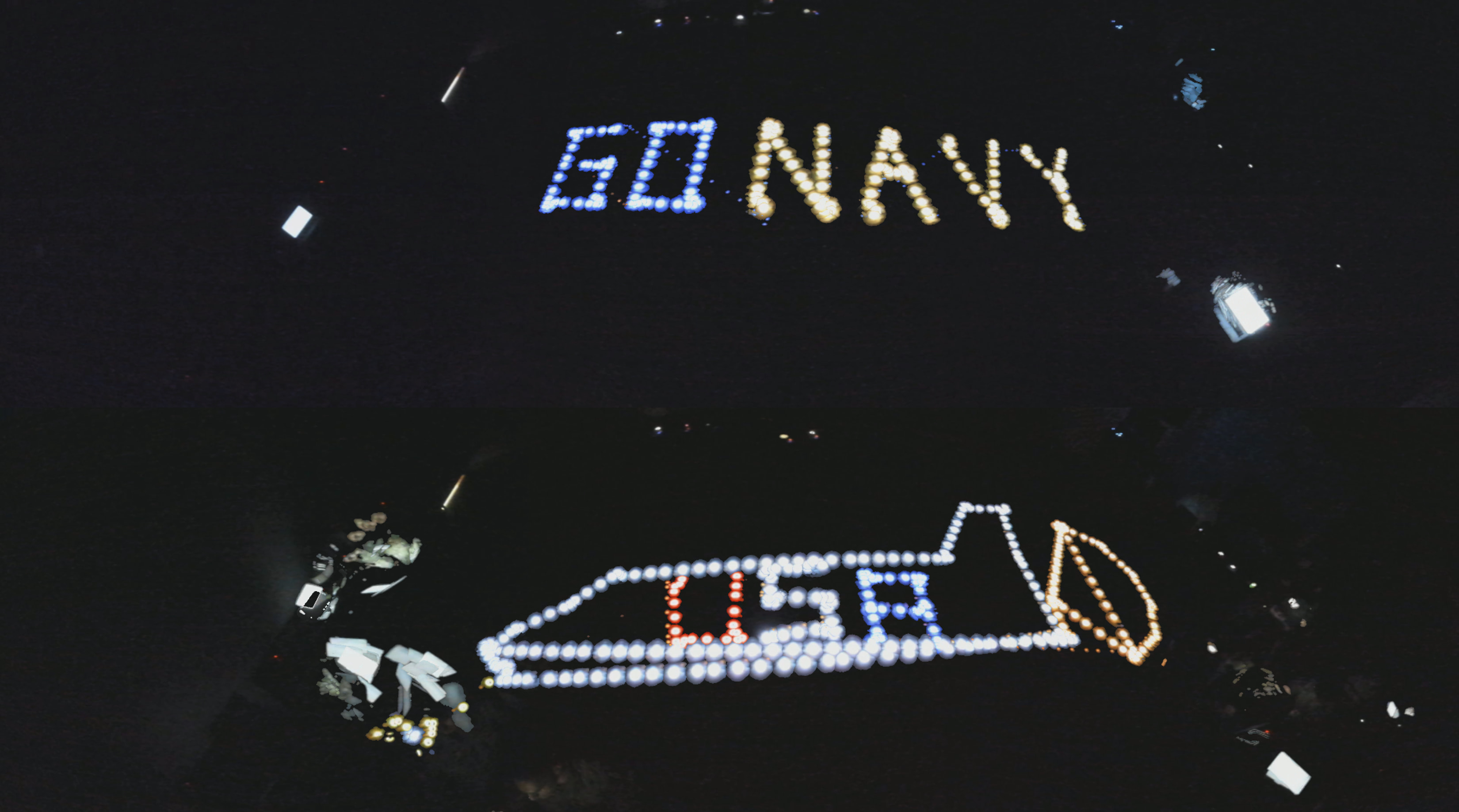
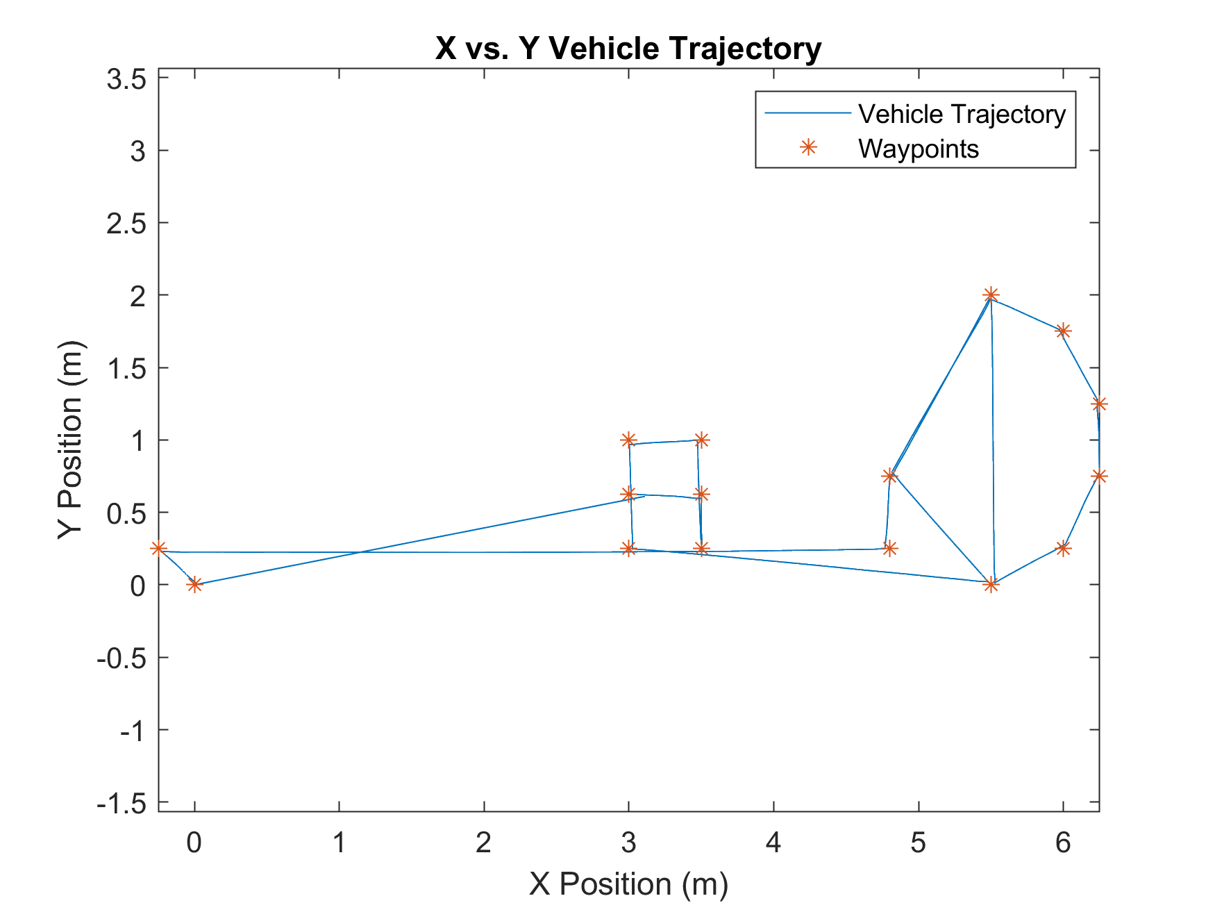
The culminating project required the programming of a generic Create3 ground vehicle to demonstrate precise waypoint control and path planning. The objective was to execute complex trajectories, visualized as a creative light display through long-exposure photography

Demo Video

Design Documentation

My final implementation involved two distinct creative outputs:

• "GO NAVY" Text: A single robot tracing the letters "GO NAVY".
• Space Shuttle: A dual-robot coordination where two vehicles simultaneously drew a space shuttle (one drew the body and the “US”, the other drew the parachute and the "A").

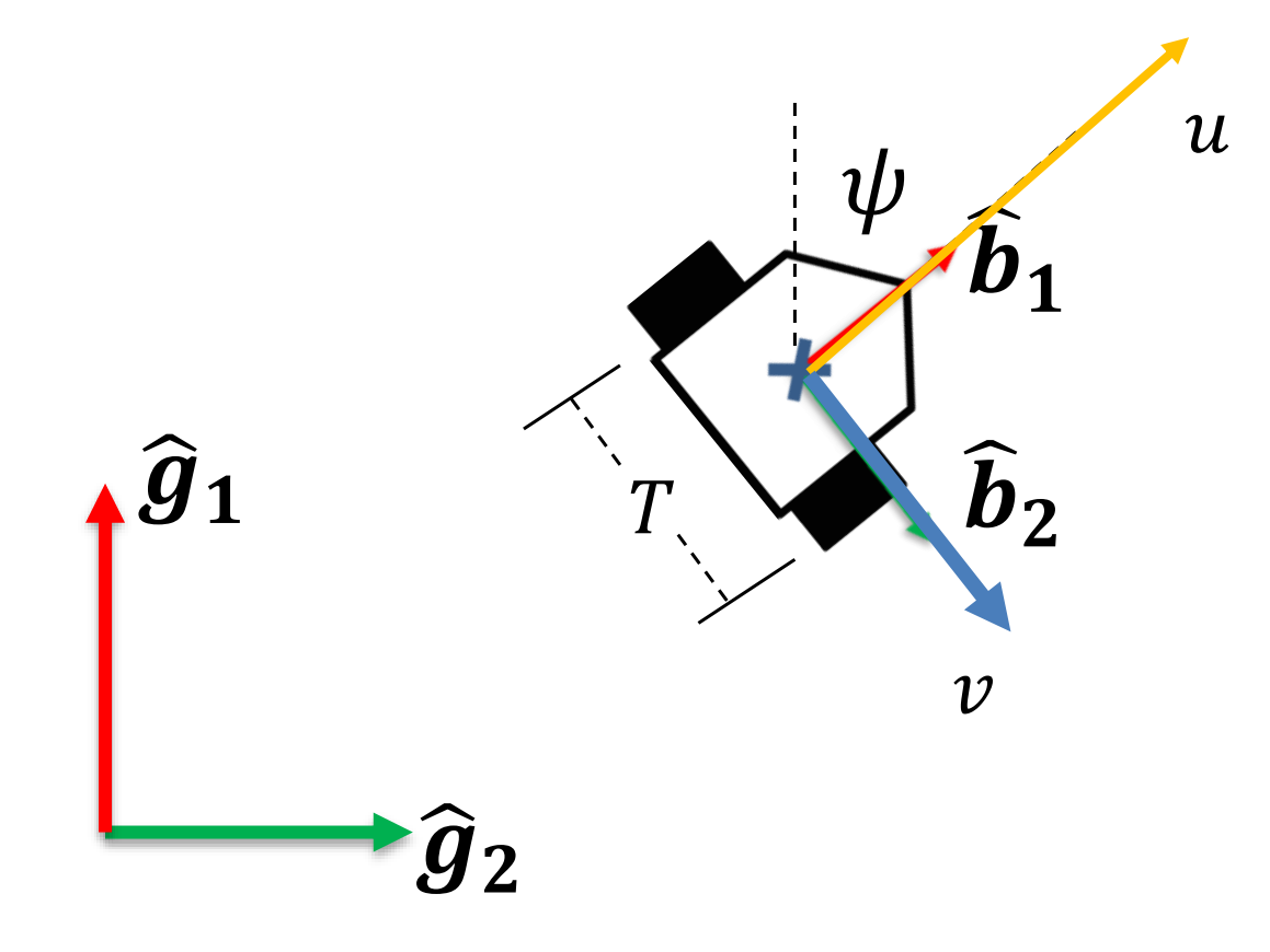
Vehicle Dynamics

To control the robot effectively, the full vehicle dynamics were analyzed in differential equation form before simplifying them for the specific implementation.

Theoretical Dynamics

The full equations of motion used are presented below.

1. Navigation Frame Positions:

$$\begin{bmatrix} \dot{x}_n \\ \dot{y}_e \\ \dot{z}_d \end{bmatrix} = \begin{bmatrix} c\psi c\theta u + (c\psi s\theta s\phi - s\psi c\phi)v + (c\psi s\theta c\phi + s\psi s\phi)w \\ s\psi c\theta u + (s\psi s\theta s\phi + c\psi c\phi)v + (s\psi s\theta c\phi - c\psi s\phi)w \\ -s\theta u + c\theta s\phi v + c\theta c\phi w \end{bmatrix}$$

2. Euler Angle Rates:

$$\begin{bmatrix} \dot{\phi} \\ \dot{\theta} \\ \dot{\psi} \end{bmatrix} = \begin{bmatrix} p + (q\sin\phi + r\cos\phi)\tan\theta \\ q\cos\phi - r\sin\phi \\ (q\sin\phi + r\cos\phi)\sec\theta \end{bmatrix}$$

3. Body Frame Velocities (Force Equations):

$$\begin{bmatrix} \dot{u} \\ \dot{v} \\ \dot{w} \end{bmatrix} = \begin{bmatrix} rv - qw + \frac{1}{m}\Sigma F_{b_1} \\ pw - ru + \frac{1}{m}\Sigma F_{b_2} \\ qu - pv + \frac{1}{m}\Sigma F_{b_3} \end{bmatrix}$$

4. Body Frame Angular Rates (Moment Equations):

$$\begin{bmatrix} \dot{p} \\ \dot{q} \\ \dot{r} \end{bmatrix} = \begin{bmatrix} \frac{I_y - I_z}{I_x}qr + \frac{1}{I_x}\Sigma M_{b_1} \\ \frac{I_z - I_x}{I_y}pr + \frac{1}{I_y}\Sigma M_{b_2} \\ \frac{I_x - I_y}{I_z}pq + \frac{1}{I_z}\Sigma M_{b_3} \end{bmatrix}$$

Simplifying Assumptions

To reduce the complexity of the model for the Create3 robot, the following assumptions were made to simplify 12 differential equations down to 3.

1. Flat Ground: The vehicle remains on the ground; therefore, pitch ($\theta$), roll ($\phi$), vertical velocity ($w$), and their rates ($\dot{p}, \dot{r}, \dot{z}, \dot{w}$) are zero.
2. No Sliding: The wheels roll without sliding, meaning lateral velocity ($v$) is zero.
3. No Slipping: Forward velocity ($u$) and turn rate ($r$) are functions of wheel speeds, assumed to have immediate stop-and-go capabilities (no inertia), meaning $\dot{u}$ and $\dot{r}$ are zero.

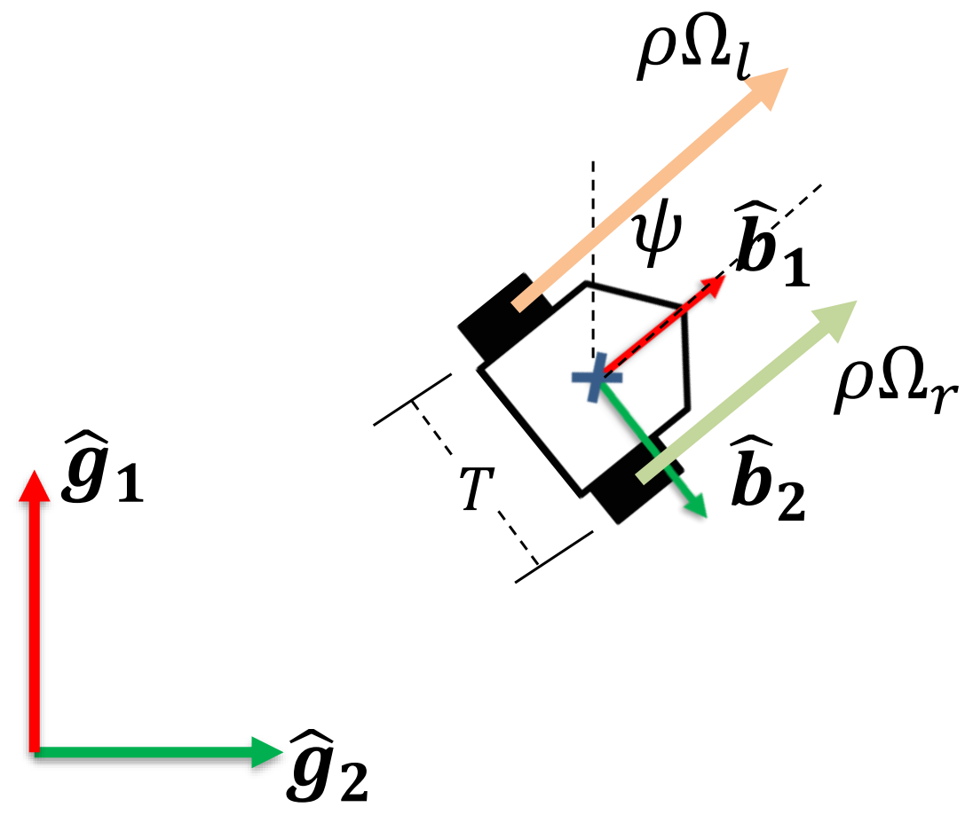
Kinematic Constraints

Based on the wheel geometry, the relationship between the wheel speeds and the vehicle's linear and angular velocity is:

$$\begin{bmatrix} u \\ r \end{bmatrix} = \begin{bmatrix} \frac{\rho}{2} & \frac{\rho}{2} \\ \frac{\rho}{T} & -\frac{\rho}{T} \end{bmatrix} \begin{bmatrix} \Omega_l \\ \Omega_r \end{bmatrix}$$

Where $\rho$ is the wheel radius and $T$ is the track width.

Final Simplified Model

The fully simplified differential equations used for the system are:

$$\begin{bmatrix} \dot{x}_n \\ \dot{y}_e \\ \dot{\psi} \end{bmatrix} = \begin{bmatrix} \cos(\psi)u \\ \sin(\psi)u \\ r \end{bmatrix}$$

Waypoint Controller Design

The Create3 robot utilizes a built-in inner loop controller to manage wheel speeds based on a desired forward velocity ($u$) and turn rate ($r$). Therefore, the project focused on developing an outer-loop controller to calculate inputs $u$ and $r$ to drive the robot toward specific global coordinates.

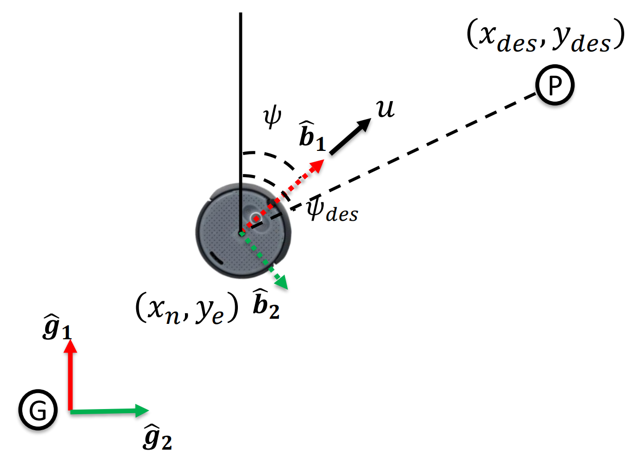
Control Logic

The controller uses Proportional Control to minimize the error between the current pose and the desired waypoint $(X_{des}, Y_{des})$. The error terms are calculated as:

$$X_{err} = X_{des} - X$$ $$Y_{err} = Y_{des} - Y$$

The desired heading ($\psi_{des}$) and distance to the target are derived from these errors:

$$\psi_{des} = \text{atan2}(Y_{err}, X_{err})$$ $$dist = \sqrt{X_{err}^2 + Y_{err}^2}$$

The control inputs are then computed using proportional gains ($K_u$ and $K_r$):

$$u = K_u \cdot dist$$ $$\psi_{err} = \psi_{des} - \psi$$ $$r = K_r \cdot \psi_{err}$$

Tuning

The gains were tuned separately. Heading ($K_r$) was tuned first to achieve static heading accuracy, followed by the speed gain ($K_u$) to optimize travel time. Inputs were saturated to stay within the robot's physical limits.

Implementation Details

Each waypoint had a set RGB light color assigned to it in an accumulated array to synchonize each waypoint with a designated color. Implemented a 0.05m tolerance radius to ensure smooth waypoint transitions and prevent the robot from backtracking. Enforced a "Turn-Then-Drive" logic where forward velocity is stopped until the heading error is reduced to within +/- 2 degrees

Waypoint Generation

"GO NAVY": Waypoints were generated using Gemini 3 Pro and copied into MATLAB.

Space Shuttle: The trajectory was manually drawn on graph paper using reference images, scaled to fit a $4 \times 6$ meter floor, and digitized into MATLAB.

Execution Logic

1. Odometry: Position estimation relied entirely on the Create3's onboard odometry.
2. Color Synchronization: Each waypoint was assigned a specific RGB light color to synchronize the LED sequence with the path.
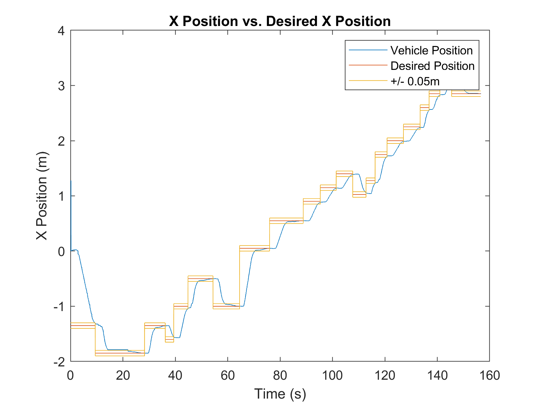
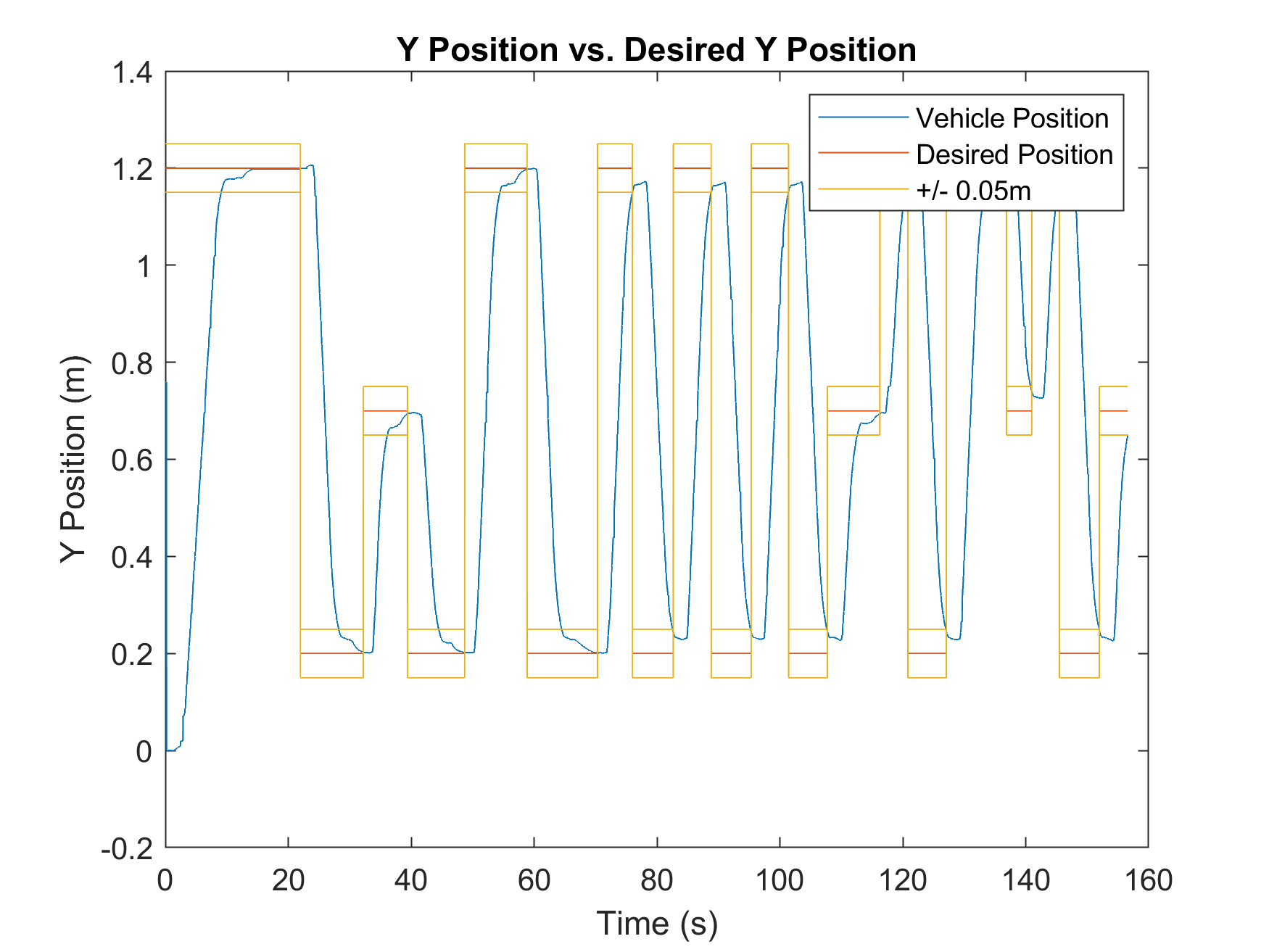
3. Tolerance: A tolerance radius of 0.05m was implemented to ensure smooth transitions without backtracking.
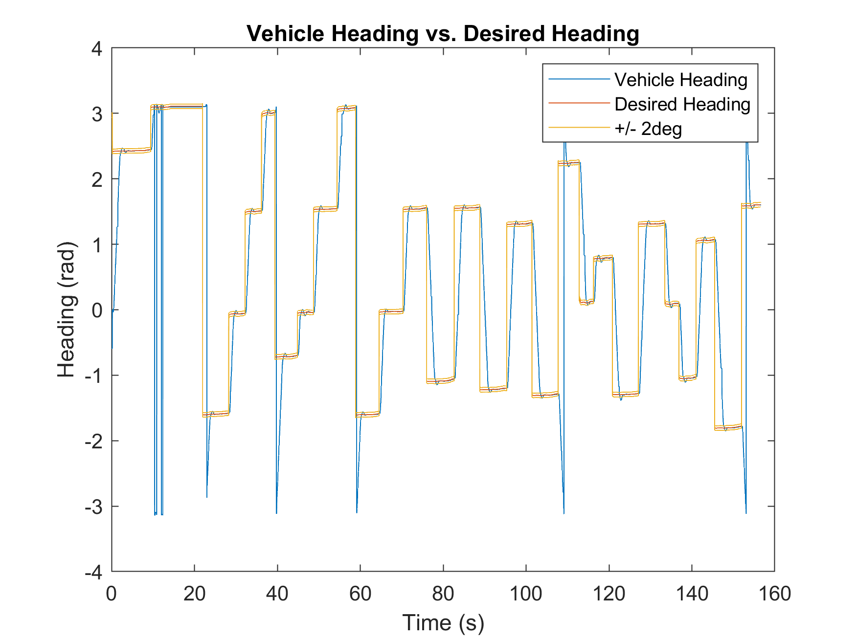
4. "Turn-Then-Drive": To improve accuracy, forward velocity is halted until the heading error is reduced to within $\pm 2^\circ$.

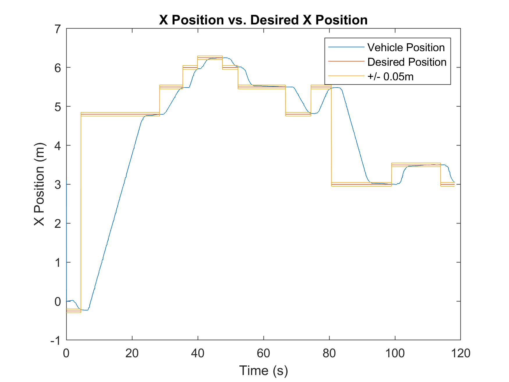
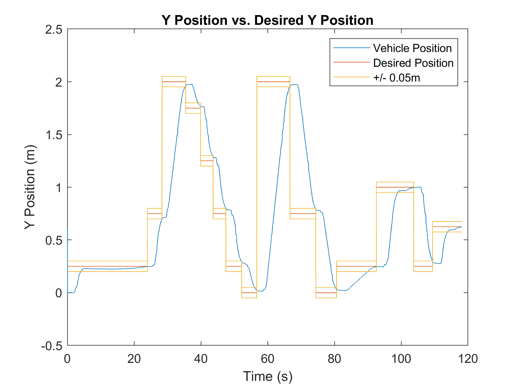
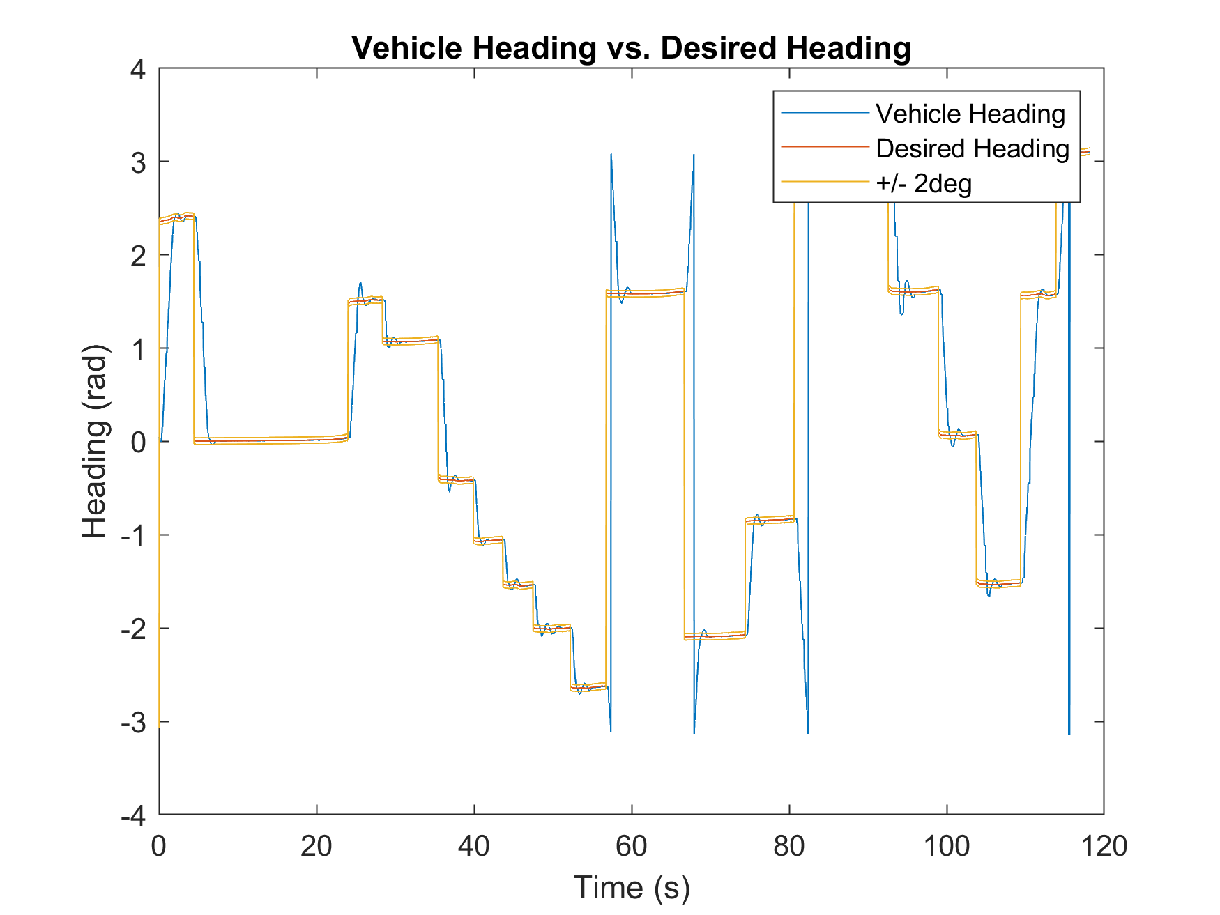
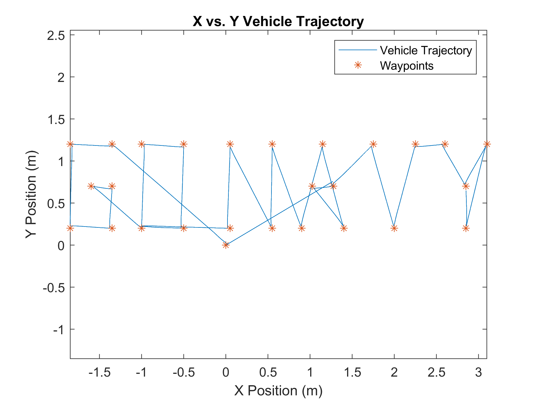
Performance Analysis

The system was verified via visual inspection and data analysis. The robot successfully achieved waypoints within the defined tolerances while executing the correct LED sequences.

Steady State Error Metrics

Metric	"GO NAVY" Pattern	Space Shuttle Pattern
X-Axis Error (m)	0.0193	0.0196
Y-Axis Error (m)	0.0283	0.0296
Heading Error (rad)	0.0046	0.0047

Both implementations showed high precision, with average position errors remaining under 3cm and heading errors under 0.005 radians.

"GO NAVY":

Space Shuttle: